Sampling (RA, dec)

Sampling the position (RA, dec) of an object on the sky is a critical for in survey-based simulation. LightCurveLynx matches the sampled positions (RA, dec) with the survey information (ObsTable) to determine when each object is observed. Points from the object’s light curve are only generated at those times where the object is observed. For example if an object is at (45.0, -10.0) and the survey includes this points at MJDs 60676.0 and 60678.0, the generated light curve will only have two fluxes. More importantly, if the sampled position falls outside the survey’s footprint the returned light curve will be empty (the object is never observed). Therefore it is critical to choose a reasonable sampling scheme.

LightCurveLynx provides multiple mechanisms for sampling object positions, including:

• Complete uniform over a sphere (UniformRADEC)

• Sampling from a survey (ObsTableRADECSampler, ObsTableUniformRADECSampler , and ApproximateMOCSampler)

• Sampling from a catalog (CatalogRADECSampler)

• Models for sampling from distributions (MilkyWayCoordSampler)

The choice of sampler will depend heavily on the science use case.

import matplotlib.pyplot as plt
import numpy as np
import pandas as pd

from lightcurvelynx.math_nodes.ra_dec_sampler import (
    ApproximateMOCSampler,
    CatalogRADECSampler,
    MilkyWayCoordSampler,
    ObsTableRADECSampler,
    ObsTableUniformRADECSampler,
    UniformRADEC,
)
from lightcurvelynx.obstable.obs_table import ObsTable
from lightcurvelynx.obstable.opsim import OpSim

/home/docs/checkouts/readthedocs.org/user_builds/lightcurvelynx/envs/stable/lib/python3.12/site-packages/tqdm/auto.py:21: TqdmWarning: IProgress not found. Please update jupyter and ipywidgets. See https://ipywidgets.readthedocs.io/en/stable/user_install.html
  from .autonotebook import tqdm as notebook_tqdm

Uniform Sampling

The simplest sampling approach is to uniformly sample (RA, dec) from the unit sphere. The UniformRADEC node does exactly this.

uniform_sampler = UniformRADEC(node_label="uniform")
(ra, dec) = uniform_sampler.generate(num_samples=500)

plt.scatter(ra, dec, s=1)
plt.show()

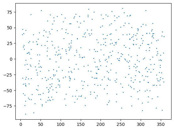
However this approach has limited use when simulating a specific survey. Depending on the survey’s coverage, a significant number of (RA, dec) points may fall outside the viewing area. In those cases, the returned light curves will be empty, indicating that there were no observations of a given object.

Sampling from a Survey’s Footprint

We can sample (RA, dec) coordinates from a survey (an ObsTable object) in two ways. First we could sample a pointing from the survey and then a point from that field of view. Second, we could sample uniformly from the region coverage by the survey.

We consider each of these approaches below, but recommend the ApproximateMOCSampler for the majority of simulations that want to generate positions from a given footprint as it is most efficient over a range of scenarios.

Sampling Pointings (Visted Weighted)

Sampling pointings from the survey provides a visit-weighted sampling of positions covered by the survey. The sampling works from a table of all the survey’s pointings and randomly selecting a row for each sample.

For concreteness let’s start with a survey that visits two fields: one centered at (45.0, -15.0) and the other at (315.0, 15.0). The first field is visited once and the second field is visited four times on four consecutive nights.

values = {
    "observationStartMJD": np.array([0.0, 1.0, 2.0, 3.0, 4.0]),
    "fieldRA": np.array([45.0, 315.0, 315.0, 315.0, 315.0]),
    "fieldDec": np.array([-15.0, 15.0, 15.0, 15.0, 15.0]),
    "zp_nJy": np.ones(5),
}
opsim = OpSim(values, radius=30.0)

We can sample from these pointings using the ObsTableRADECSampler node.

pointing_sampler = ObsTableRADECSampler(opsim, radius=10.0, node_label="opsim")
(ra, dec, time) = pointing_sampler.generate(num_samples=100)

plt.scatter(ra, dec, s=1)
plt.show()

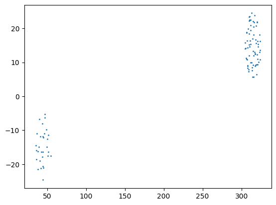
As we can see, the field centered in the Northern hemisphere is sampled significantly more than the one centered in the Southern hemisphere, because the survey visited that field more often.

Users can limit the overlap with the dedup_threshold parameter, which removes near duplicate rows. But for non-visit-weighted sampling of a survey, we highly recommend using one of either ObsTableUniformRADECSampler or ApproximateMOCSampler.

Sampling Survey Coverage

If we instead would like to sample uniformly from the area covered by the survey, we have two options (ObsTableUniformRADECSampler and ApproximateMOCSampler) with different trade offs.

ObsTableUniformRADECSampler

The ObsTableUniformRADECSampler uses rejection sampling to generate positions. This means that for every sampled position it randomly guesses an (RA, dec) then checks if that point falls within the survey. If not, it repeats the process until it finds a valid point or reaches max_iterations iterations (at which point it returns the last sample). This approach works well for surveys with significant coverage.

coverage_sampler1 = ObsTableUniformRADECSampler(opsim, radius=30.0, node_label="coverage1")
(ra, dec) = coverage_sampler1.generate(num_samples=100)

plt.scatter(ra, dec, s=1)
plt.show()

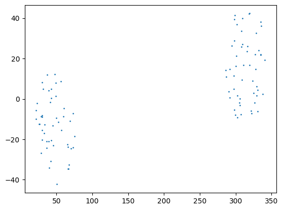
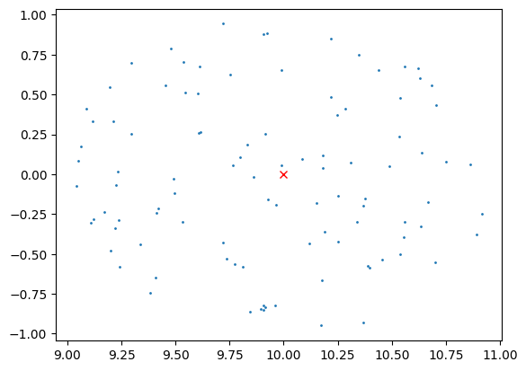
The ObsTableUniformRADECSampler does not perform well for surveys with small coverage. In the best case it may take many guesses to get find a point within the survey. In the worst, case all max_iterations fail and the sampler returns a random point outside the survey.

values = {
    "time": np.array([0.0]),
    "ra": np.array([10.0]),
    "dec": np.array([0.0]),
    "zp": np.ones(1),
}
ops_data = ObsTable(values)

coverage_sampler2 = ObsTableUniformRADECSampler(ops_data, radius=1.0, node_label="coverage2")
(ra, dec) = coverage_sampler2.generate(num_samples=100)

plt.scatter(ra, dec, s=1)
plt.plot(10.0, 0.0, "rx")
plt.show()

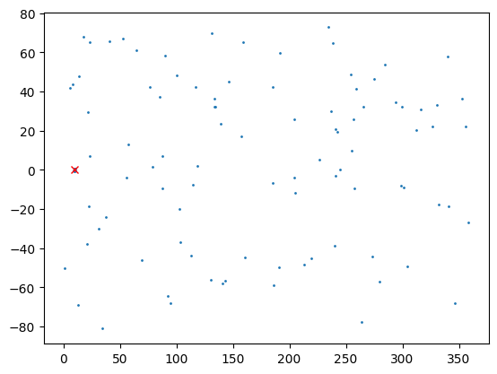
As you can see, many of the points land outside the 1 degree radius around the center of the pointing (10, 0).

We recommend the ObsTableUniformRADECSampler only for cases where there is large survey coverage.

ApproximateMOCSampler

The ApproximateMOCSampler samples from the area covered by a Multi-Order Coverage Map (MOC), which is a collection of healpix pixels representing an area on the sky. Users can generate custom MOCs for hypothetical surveys, build a MOC from a survey, or use a helper function to create the sampler directly from the survey. This is our recommended approach for sampling from a survey.

We show an example using the from_obstable helper function.

coverage_sampler3 = ApproximateMOCSampler.from_obstable(
    ops_data,
    radius=1.0,
    node_label="coverage3",
    depth=14,
)
(ra, dec) = coverage_sampler3.generate(num_samples=100)

plt.scatter(ra, dec, s=1)
plt.plot(10.0, 0.0, "rx")
plt.show()

as we can see the sample points all fall within 1.0 degree of the center of the pointing (10, 0).

This sampling is approximate, because depending on the depth of the MOC, the healpix tiles used to cover the survey might include area outside the survey. You can tradeoff accuracy with compute cost (run time and memory) using the depth parameter. (Note that is you generate the MOC separately, you will need to define a max depth during that operation as well).

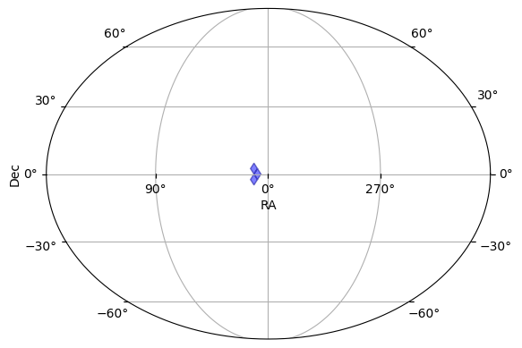
We can look at the footprint covered by the sampler using the built-in plot_footprint() function.

_ = coverage_sampler3.plot_footprint()

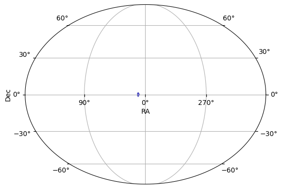
For example, if we use depth=8, the survey’s coverage is approximated by a grid of only 786,432 pixels over the entire sky with (an average pixel width of around 14 arc minutes). We recommend at least a depth of 12 (average pixel width around 50 arc seconds) for reasonable accuracy.

As a concrete example, let’s look at what happens if we prebuild the MOC at depth=4 (very coarse). Although the sampler uses a depth of 14, it cannot extract any more resolution from the input than it was given (a depth=4 MOC).

# Manually build a very coarse MOC.
moc = ops_data.build_moc(radius=1.0, max_depth=4)
coverage_sampler3 = ApproximateMOCSampler(moc, depth=14, node_label="coverage3")
coverage_sampler3.plot_footprint()

(<Figure size 640x480 with 1 Axes>, <WCSAxes: >)

Because of the coarse approximation, the sampled data now contains many points outside the survey’s radius.

Both the manual construction of a MOC from the ObsTable and the ApproximateMOCSampler.from_obstable helper function can account for the detector footprint (if one is provided) by setting the argument use_footprint=True.

The ApproximateMOCSampler also support building samplers from multiple survey footprints:

• ApproximateMOCSampler.from_obstable_union() build the sampling footprint from the union of the survey footprints.

• ApproximateMOCSampler.from_obstable_intersection() build the sampling footprint from the intersection of the survey footprints.

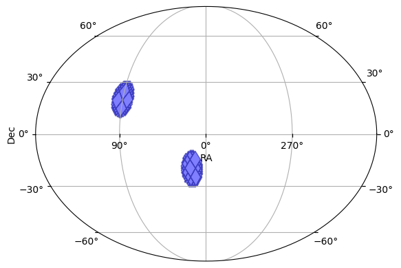
In addition, users can create their own MOC of the sampling area and pass that directly into the sampler’s constructor.

from astropy.coordinates import Latitude, Longitude
import astropy.units as u
from mocpy import MOC

longitudes = Longitude([15.0, 90.0], unit="deg")
latitudes = Latitude([-20.0, 20.0], unit="deg")
moc = MOC.from_cones(
    lon=longitudes,
    lat=latitudes,
    radius=10.0 * u.deg,
    max_depth=12,
    union_strategy="large_cones",
)
moc_sampler = ApproximateMOCSampler(moc)
moc_sampler.plot_footprint()

(<Figure size 640x480 with 1 Axes>, <WCSAxes: >)

Sampling from a Catalog

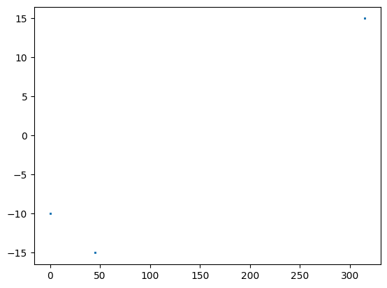
We can use the CatalogRADECSampler node to sample from a catalog of known objects. This class is a thin connivence wrapper on the ObsTableRADECSampler that samples only ra and dec and defaults to a zero radius (exact sampling of observations). It provides a dedup_threshold parameter for removing near duplicates.

# 4 points with one pair of duplicates
values = {
    "ra": np.array([45.0, 315.0, 315.0, 0.0]),
    "dec": np.array([-15.0, 15.0, 15.0, -10.0]),
}
data = pd.DataFrame(values)

pointing_sampler = CatalogRADECSampler(data, dedup_threshold=0.1, node_label="catalog")
print(f"The sampler will draw from {len(pointing_sampler)} points.")

(ra, dec) = pointing_sampler.generate(num_samples=100)

plt.scatter(ra, dec, s=1)
plt.show()

The sampler will draw from 3 points.

We can use the CatalogRADECSampler (as well as the ObsTableRADECSampler) includes a from_hats() function that allows users to directly load a catalog from the HATS format.

Sampling from a Model Distribution

We can use built-in or custom defined distribution models for more specific sampling cases. As one example, consider the MilkyWayCoordSampler which samples from density distribution of the milky way. Below we use the density model defined in Juric et al., 2008, but users can also define their own models.

from lightcurvelynx.astro_utils.milky_way_density import MilkyWayDensityJuric2008

density_model = MilkyWayDensityJuric2008()
pointing_sampler = MilkyWayCoordSampler(density_model=density_model)
(ra, dec, dist_pc) = pointing_sampler.generate(num_samples=1000)

plt.scatter(ra, dec, s=1)
plt.show()

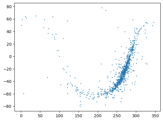
Note that as shown in the example, we can define samplers that produce more than just RA, dec. The MilkyWayCoordSampler also returns a distance in parsecs.

Linking (RA, dec) to Models

To be useful, the (RA, dec) locations that we generate must be linked into our model objects. To support this all the generators above produce a pair of named outputs “ra” and “dec”. This means we can use LightCurveLynx’s reference functionality to set the object’s position based on the samples.

from lightcurvelynx.models.basic_models import ConstantSEDModel

model = ConstantSEDModel(
    ra=uniform_sampler.ra,
    dec=uniform_sampler.dec,
    brightness=100.0,
    node_label="source",
)
state = model.sample_parameters(num_samples=10)
print(state)

uniform:
    ra: [ 68.20597776 254.69425749  57.37977518 235.80707771 233.27106996
 161.6077301  262.19908986 330.43000074 245.32943044 231.29920369]
    dec: [-84.24607546 -10.82880461  19.15533906   6.5705303  -52.32266261
  59.49064026  35.70756062  18.39841786  10.66368179  53.15010807]
source:
    ra: [ 68.20597776 254.69425749  57.37977518 235.80707771 233.27106996
 161.6077301  262.19908986 330.43000074 245.32943044 231.29920369]
    dec: [-84.24607546 -10.82880461  19.15533906   6.5705303  -52.32266261
  59.49064026  35.70756062  18.39841786  10.66368179  53.15010807]
    redshift: [None None None None None None None None None None]
    t0: [None None None None None None None None None None]
    distance: [None None None None None None None None None None]
    brightness: [100. 100. 100. 100. 100. 100. 100. 100. 100. 100.]

Handling Multiple Surveys

Currently the only sampling approach that can handle multiple surveys is the ApproximateMOCSampler. That class contains built-in constructor methods for creating a sampling footprint from either the union or intersection of footprints of the individual surveys.

Positions Outside the Surveys

When the positional sampler includes positions outside the survey’s footprint, the simulation will occasionally draw an (RA, dec) that is not observed at any times. As a result, no data will be simulated and the results table will include a row with an empty light curve. This is the most common reason for empty light curves. The user can either refine the bounds of the sampler (such as increasing the MOC depth) or just filter out the unobserved points.