Simulating Combinations of Objects

For some extragalatic studies, the user might be interested in simulating the combination of fluxes coming from multiple objects. The simplest case of this is an object and its host galaxy. However, other combinations, such as two blended objects, use the same mechanism.

LightCurveLynx provides a general purpose class AdditiveMultiObjectModel that produces the combined flux densities from multiple models. This class can be used to simulate host/object combinations, unresolved sources, etc.

The AdditiveMultiObjectModel Node

The AdditiveMultiObjectModel node model takes a list of BasePhysicalModel objects and returns the sum of their flux densities. As an example, let’s create a source that is a sinwave (with magnitude 3.0) in front of a static host (of brightness 5).

import numpy as np

from lightcurvelynx.models.basic_models import SinWaveModel, ConstantSEDModel
from lightcurvelynx.models.multi_object_model import AdditiveMultiObjectModel

host = ConstantSEDModel(
    brightness=5.0,
    ra=10.0,
    dec=-5.0,
)

source = SinWaveModel(
    amplitude=3.0,
    frequency=1.0,
    t0=0.0,
    ra=10.01,
    dec=-5.01,
)

model = AdditiveMultiObjectModel(objects=[source, host])

/home/docs/checkouts/readthedocs.org/user_builds/lightcurvelynx/envs/stable/lib/python3.12/site-packages/tqdm/auto.py:21: TqdmWarning: IProgress not found. Please update jupyter and ipywidgets. See https://ipywidgets.readthedocs.io/en/stable/user_install.html
  from .autonotebook import tqdm as notebook_tqdm

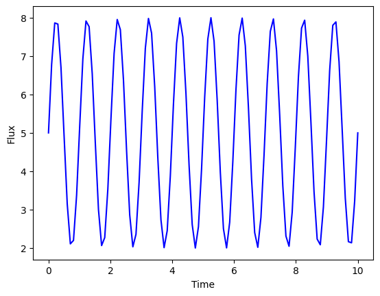
Next we evaluate the combined model across a range of times. As we see, the fluxes oscillate from [-3, 3] against a background of 5.

import matplotlib.pyplot as plt

times = np.linspace(0, 10, 100)
wavelengths = np.array([500])

fluxes = model.evaluate_sed(times, wavelengths)

plt.plot(times, fluxes[:, 0], color="blue")
plt.xlabel("Time")
plt.ylabel("Flux")
plt.show()

RA, dec, and Other Parameters

It is important to note that the AdditiveMultiObjectModel node does not automatically inherit any of the parameters from its objects. It also does not ensure that any of the values, such as position, are the same.

This is intentional to allow the component objects to vary. For example we might want a star that is offset from the center of the host (ra_star != ra_host and dec_star != dec_host). Or we may want two unresolved sources at completely different redshifts.

print(model.sample_parameters())

SinWaveModel_1:
    ra: 10.01
    dec: -5.01
    redshift: None
    t0: 0.0
    distance: None
    brightness: 0.0
    amplitude: 3.0
    frequency: 1.0
ConstantSEDModel_2:
    ra: 10.0
    dec: -5.0
    redshift: None
    t0: None
    distance: None
    brightness: 5.0
AdditiveMultiObjectModel_0:
    ra: None
    dec: None
    redshift: None
    t0: None
    distance: None

In order to ensure the final computations include RA, dec, etc. it is necessary to specify them as arguments when creating the additive mode itself. LightCurveLynx uses these parameters of the object passed into the simulation stage: a) to determine when each object is observed (given the pointings in an ObsTable), and b) to record in the result table. It is important to note that, when using an AdditiveMultiObjectModel, the RA and dec (and other parameters) saved will be the one assigned to the outer-most object.

If you want to use the same (RA, dec) as one of the components, you can access that object’s parameter value with the dot notation. For example, in a host/source model, most users will want the model’s RA and dec (and redshift) to correspond to that of the source.

Remember from the sampling notebook that this links the parameters so that the values of the two objects will be consistent within each iteration of the simulation.

model = AdditiveMultiObjectModel(
    objects=[source, host],
    ra=source.ra,
    dec=source.dec,
)
print(model.sample_parameters())

SinWaveModel_1:
    ra: 10.01
    dec: -5.01
    redshift: None
    t0: 0.0
    distance: None
    brightness: 0.0
    amplitude: 3.0
    frequency: 1.0
ConstantSEDModel_2:
    ra: 10.0
    dec: -5.0
    redshift: None
    t0: None
    distance: None
    brightness: 5.0
AdditiveMultiObjectModel_0:
    ra: 10.01
    dec: -5.01
    redshift: None
    t0: None
    distance: None

Alternately you might sample a single position (RA, dec) and use it for all the objects. The “sampling_positions” notebook provides a deep dive into the different spatial samplers included with LightCurveLynx.

from lightcurvelynx.math_nodes.ra_dec_sampler import UniformRADEC

uniform_sampler = UniformRADEC(node_label="uniform")

host = ConstantSEDModel(
    brightness=5.0,
    ra=uniform_sampler.ra,
    dec=uniform_sampler.dec,
)

source = SinWaveModel(
    amplitude=3.0,
    frequency=1.0,
    t0=0.0,
    ra=uniform_sampler.ra,
    dec=uniform_sampler.dec,
)

model = AdditiveMultiObjectModel(
    objects=[source, host],
    ra=uniform_sampler.ra,
    dec=uniform_sampler.dec,
)

Redshift and Effects

Redshift and rest frame effects are applied to each object individually (to allow for unresolved sources at different redshifts). In contrast, observer frame effects are applied to the combination of fluxes. From the user’s point of view, effects can be added to the AdditiveMultiObjectModel the same way as any other model. The model will internally handle how these effects are applied.

from lightcurvelynx.effects.basic_effects import ScaleFluxEffect

# Create a dimming effect (in the rest frame) and add it to the model.
dimming = ScaleFluxEffect(flux_scale=0.5, rest_frame=True)
model.add_effect(dimming)

fluxes = model.evaluate_sed(times, wavelengths)

plt.plot(times, fluxes[:, 0], color="blue")
plt.xlabel("Time")
plt.ylabel("Flux")
plt.show()

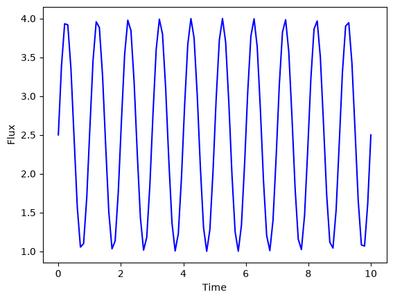
As we can see the contributions of both the host and object are dimmed.