Extrapolation

While some models are defined over all possible times and wavelengths, other models might only be defined within a set range. Consider a model that is defined by an underlying spline over a grid of predicted fluxes at different times and wavelengths. Within the grid of times and wavelengths, the model may be very accurate. But, depending on the model, things could look bad if you try to query points outside this range.

Similar problems arise with bandflux models fit from real observations. What do you do for times outside the observed range?

In this notebook we show how LightcurveLynx provides different extrapolation options for dealing with these types of cases.

Valid Bounds

LightCurveLynx uses the same functions as sncosmo:

• Time bounds are returned in days relative to t0 by a pair of functions minphase() and maxphase()

• Wavelength bounds are returns in Angstroms by a pair of functions minwave() and maxwave()

For models such as the SncosmoWrapperModel or the LightcurveTemplateModel these bounds are automatically defined by the underlying data or model. For user defined models, a user can include the bounds directly. Let’s consider a sine-wave based model that is only defined over times [t0 - 50, t0 + 100] and wavelengths [1,000, 10,000].

import numpy as np

from lightcurvelynx.models.physical_model import SEDModel


class BoundedSinModel(SEDModel):
    """A model that emits a sine wave:

    flux = brightness * sin(2 * pi * frequency * (time - t0))

    defined for times in [t0 - 50, t0 + 100] and wavelengths in [1000, 10000].

    Parameters
    ----------
    brightness : `float`
        The inherent brightness
    frequency : `float`
        The frequence of the sine wave.
    **kwargs : `dict`, optional
        Any additional keyword arguments.
    """

    def __init__(self, brightness, frequency, **kwargs):
        super().__init__(**kwargs)
        self.add_parameter(
            "brightness",
            brightness,
            description="The inherent brightness",
        )
        self.add_parameter(
            "frequency",
            frequency,
            description="The frequency of the sine wave.",
        )

    def minwave(self, **kwargs):
        """The minimum wavelength for this model."""
        return 1000.0

    def maxwave(self, **kwargs):
        """The maximum wavelength for this model."""
        return 10000.0

    def minphase(self, **kwargs):
        """The minimum phase for this model."""
        return -50.0

    def maxphase(self, **kwargs):
        """The maximum phase for this model."""
        return 100.0

    def compute_sed(self, times, wavelengths, graph_state, **kwargs):
        """Draw effect-free observations for this object.

        Parameters
        ----------
        times : `numpy.ndarray`
            A length T array of rest frame timestamps.
        wavelengths : `numpy.ndarray`, optional
            A length N array of wavelengths (in angstroms).
        graph_state : `GraphState`
            An object mapping graph parameters to their values.
        **kwargs : `dict`, optional
            Any additional keyword arguments.

        Returns
        -------
        flux_density : `numpy.ndarray`
            A length T x N matrix of SED values (in nJy).
        """
        params = self.get_local_params(graph_state)
        phase = times - params["t0"]

        if np.any(wavelengths < self.minwave()) or np.any(wavelengths > self.maxwave()):
            raise ValueError("Invalid wavelengths.")
        if np.any(phase < self.minphase()) or np.any(phase > self.maxphase()):
            raise ValueError("Invalid times.")

        phases = 2.0 * np.pi * params["frequency"] * phase
        single_wave = params["brightness"] * np.sin(phases)
        return np.tile(single_wave[:, np.newaxis], (1, len(wavelengths)))


model = BoundedSinModel(brightness=15.0, frequency=0.031415, t0=0.0)

/home/docs/checkouts/readthedocs.org/user_builds/lightcurvelynx/envs/stable/lib/python3.12/site-packages/tqdm/auto.py:21: TqdmWarning: IProgress not found. Please update jupyter and ipywidgets. See https://ipywidgets.readthedocs.io/en/stable/user_install.html
  from .autonotebook import tqdm as notebook_tqdm

As long as we evaluate the model in the given range, everything is good.

import matplotlib.pyplot as plt

times = np.linspace(-50, 100, 100)
wavelengths = np.array([5000.0])
values = model.evaluate_sed(times, wavelengths)
plt.plot(times, values[:, 0])
plt.xlabel("Phase (days)")
plt.ylabel("Flux Density (nJy)")

Text(0, 0.5, 'Flux Density (nJy)')

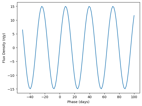
But if we were to try to evaluate a point outside either the time or wavelength bounds, we would have a problem. In this case the problem is pretty obvious. The program fails. But for other models, we might see cases of bad extrapolation or zero padding that give unrealistic results.

times = np.arange(-100, 200)
wavelengths = np.array([5000.0])

try:
    values = model.evaluate_sed(times, wavelengths)
except ValueError as e:
    print("Failed with error:", e)

Failed with error: Invalid times.

/home/docs/checkouts/readthedocs.org/user_builds/lightcurvelynx/envs/stable/lib/python3.12/site-packages/lightcurvelynx/models/physical_model.py:535: UserWarning: Some times are less than the model's defined bounds and no time extrapolation is set. If this is not the intended, you can enable time extrapolation using the 'time_extrapolation' parameter.
  warnings.warn(
/home/docs/checkouts/readthedocs.org/user_builds/lightcurvelynx/envs/stable/lib/python3.12/site-packages/lightcurvelynx/models/physical_model.py:562: UserWarning: Some times are greater than the model's defined bounds and no time extrapolation is set. If this is not the intended, you can enable time extrapolation using the 'time_extrapolation' parameter.
  warnings.warn(

As shown above models will also provide warnings when queried outside their valid range. While this may be redundant if the model fails (like the BoundedSinModel), it is useful to know if the model is attempting its own implicit extrapolation (such as with a general spline).

Extrapolation

LightcurveLynx provides a variety of models (in the form of FluxExtrapolationModel objects) that can be used to extrapolate beyond the valid bounds. These objects are passed to the model during construction using the arguments time_extrapolation and wave_extrapolation.

Each of those arguments can either be a FluxExtrapolationModel object or a length 2 tuple of such objects. If a pair of objects if given first one is used for extrapolation before the valid range and the second is used for extrapolation after the valid range. If only a single object is provided, it is used for extrapolation before and after the range.

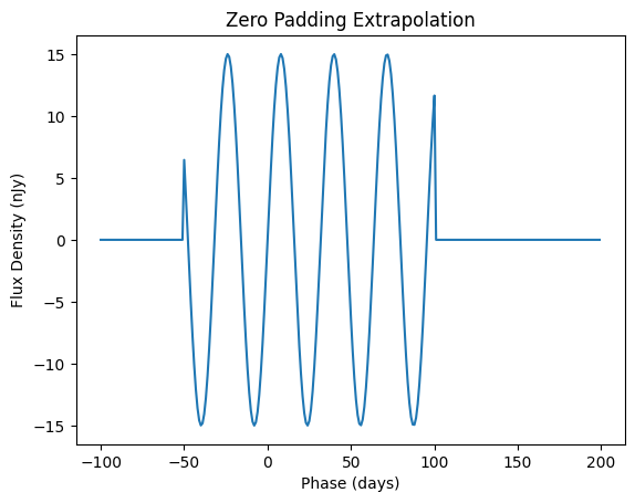
Zero Padding

The simplest extrapolation strategy is zero padding, which just adds zeros outside the valid range.

from lightcurvelynx.utils.extrapolate import ZeroPadding

model = BoundedSinModel(brightness=15.0, frequency=0.031415, t0=0.0, time_extrapolation=ZeroPadding())
values = model.evaluate_sed(times, wavelengths)

plt.plot(times, values[:, 0])
plt.xlabel("Phase (days)")
plt.ylabel("Flux Density (nJy)")
plt.title("Zero Padding Extrapolation")
plt.show()

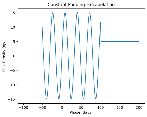
Constant Padding

We can also pad the invalid range with other (user-defined) constant values.

from lightcurvelynx.utils.extrapolate import ConstantPadding

before_extrap = ConstantPadding(10.0)
after_extrap = ConstantPadding(5.0)

model = BoundedSinModel(
    brightness=15.0, frequency=0.031415, t0=0.0, time_extrapolation=(before_extrap, after_extrap)
)
values = model.evaluate_sed(times, wavelengths)

plt.plot(times, values[:, 0])
plt.xlabel("Phase (days)")
plt.ylabel("Flux Density (nJy)")
plt.title("Constant Padding Extrapolation")
plt.show()

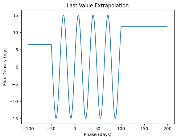
Last Value Extrapolation

The LastValue class simply propogates the last valid value output by the function in that direction.

from lightcurvelynx.utils.extrapolate import LastValue

model = BoundedSinModel(brightness=15.0, frequency=0.031415, t0=0.0, time_extrapolation=LastValue())
values = model.evaluate_sed(times, wavelengths)

plt.plot(times, values[:, 0])
plt.xlabel("Phase (days)")
plt.ylabel("Flux Density (nJy)")
plt.title("Last Value Extrapolation")
plt.show()

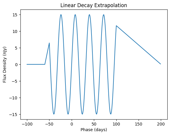
Linear Decay Extrapolation

The LinearDecay class starts the flux at the last value and ramps it down linearly over a given time window.

from lightcurvelynx.utils.extrapolate import LinearDecay

before_extrap = LinearDecay(10.0)
after_extrap = LinearDecay(100.0)

model = BoundedSinModel(
    brightness=15.0, frequency=0.031415, t0=0.0, time_extrapolation=(before_extrap, after_extrap)
)
values = model.evaluate_sed(times, wavelengths)

plt.plot(times, values[:, 0])
plt.xlabel("Phase (days)")
plt.ylabel("Flux Density (nJy)")
plt.title("Linear Decay Extrapolation")
plt.show()

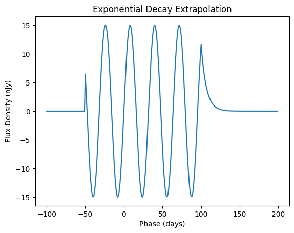
Exponential Decay Extrapolation

The ExponentialDecay class starts the flux at the last value and ramps it down exponentially given a decay rate:

from lightcurvelynx.utils.extrapolate import ExponentialDecay

before_extrap = ExponentialDecay(10.0)
after_extrap = ExponentialDecay(0.15)

model = BoundedSinModel(
    brightness=15.0, frequency=0.031415, t0=0.0, time_extrapolation=(before_extrap, after_extrap)
)
values = model.evaluate_sed(times, wavelengths)

plt.plot(times, values[:, 0])
plt.xlabel("Phase (days)")
plt.ylabel("Flux Density (nJy)")
plt.title("Exponential Decay Extrapolation")
plt.show()

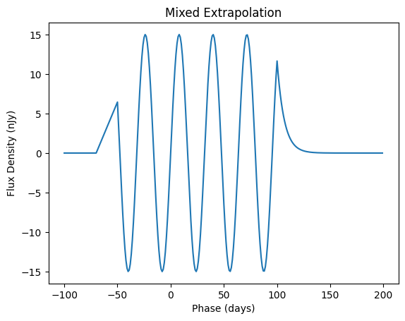
Combining Types

Of course users might want to use different extrapolation functions before and after the valid ranges. This can be done by passing in different types of objects. None can be passed in for either object in order to perform no extrapolation in that direction. Instead the model is queried directly with the points outside its range.

before_extrap = LinearDecay(20.0)
after_extrap = ExponentialDecay(0.15)

model = BoundedSinModel(
    brightness=15.0, frequency=0.031415, t0=0.0, time_extrapolation=(before_extrap, after_extrap)
)
values = model.evaluate_sed(times, wavelengths)

plt.plot(times, values[:, 0])
plt.xlabel("Phase (days)")
plt.ylabel("Flux Density (nJy)")
plt.title("Mixed Extrapolation")
plt.show()

Bandflux Models

Bandflux models support time extrapolation using the same mechanism. However they do not support wavelength extrapolation because they do not make predictions at the wavelength level. If you try to provide a wavelength extrapolation argument to a bandflux only model, it will show a warning.