Passband Demo
A Passband object stores the information needed to transform the observed flux density over multiple wavelengths into a single band flux for a given filter. A PassbandGroup object implements a collection of Passband objects providing convenient helper functions for loading and processing multiple passbands.
By default the passband data files are stored in the data/passbands subdirectory of the top level LightCurveLynx directory.
[1]:
import math

import matplotlib.pyplot as plt
import numpy as np

from pathlib import Path

from lightcurvelynx.astro_utils.passbands import Passband, PassbandGroup
from lightcurvelynx.utils.plotting import plot_bandflux_lightcurves, plot_flux_spectrogram

# Usually we would not hardcode the path to the passband files, but for this demo we will use a relative path
# to the test data directory so that we do not have to download the files.
table_dir = "../../tests/lightcurvelynx/data/passbands"
/home/docs/checkouts/readthedocs.org/user_builds/lightcurvelynx/envs/stable/lib/python3.12/site-packages/tqdm/auto.py:21: TqdmWarning: IProgress not found. Please update jupyter and ipywidgets. See https://ipywidgets.readthedocs.io/en/stable/user_install.html
  from .autonotebook import tqdm as notebook_tqdm
Passband Example
Let’s start with looking at a simple Passband and the information it contains. As we will see below, the Passband class provides multiple mechanisms for loading in the passband information, including reading it in from both ASCII and VOTable files.
Loading from a File
If we have the passband’s file downloaded, we can load it with the Passband.from_file() function. Here we open the g-band information from the LSST files in our testing directory.
[2]:
lsst_g = Passband.from_file(
    "LSST",  # The survey name
    "g",  # The filter name
    table_path=Path(table_dir, "LSST", "g.dat"),  # The path to the passband file
)
lsst_g.plot()
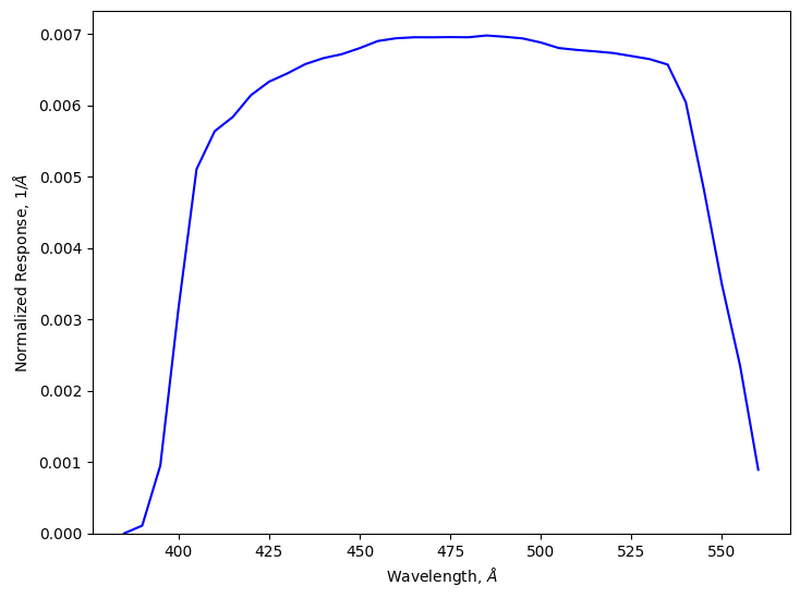
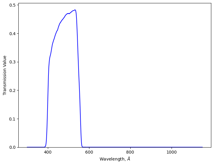
By default the plotting function will plot the normalized response. Alternatively, we could plot the loaded transmission curve.
[3]:
lsst_g.plot(plot_transmission=True)
Downloading Files
Both Passband.from_file() can take a combination of file path and URL information. LightCurveLynx uses the pooch library to handle downloading files and maintaining versions. If the file in the given path already exists, it will be used directly. Otherwise pooch will download it to that location. We could specify a URL from which to download the files with the table_url parameter.
Note: Throughout this notebook, we use the hardcoded test directory path to retrieve pre-downloaded files so the notebook does not have external dependencies. In most cases, users will want to use the default table directory (data/passbands) and let LightCurveLynx handle the downloads and caching.
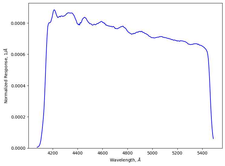
A special case of the file download is retrieving passbands from the SVO filter profile service. LightCurveLynx includes a built in function Passband.from_svo() that takes the SVO identifier and uses astroquery to download the data.
Let’s look at the ‘g’ filter from the ZTF survey.
[4]:
ztf_g = Passband.from_svo("Palomar/ZTF.g")
ztf_g.plot()
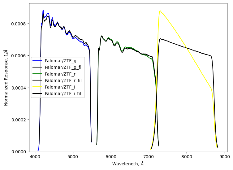
Or you can download ALL the filters for a facility and instrument by just providing that information to PassbandGroup.from_svo(). Under the hood, this function uses astroquery.svo_fps.SvoFps.get_filter_list() which takes a facility and instrument. So the string should be “{FACILITY}/{INSTRUMENT}”.
[5]:
pbg = PassbandGroup.from_svo("Palomar/ZTF")
pbg.plot()
Manually specified passbands
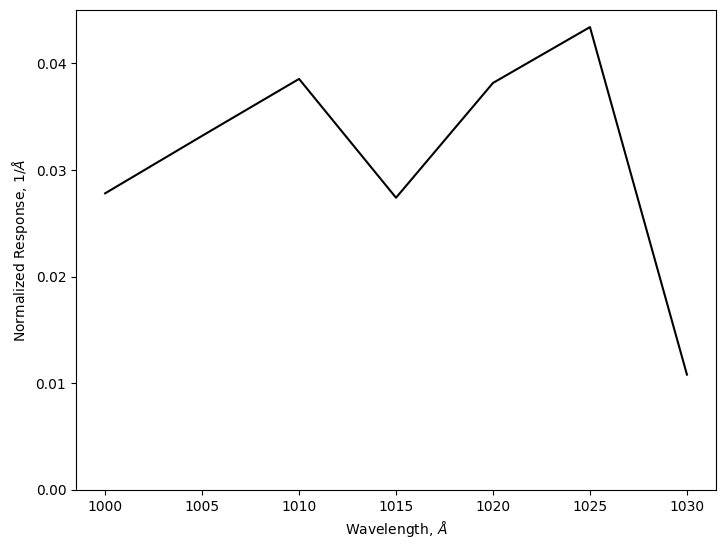
For testing, we might want to manually specify the passband information. We can do this by creating a 2-dimensional numpy array where the first column is wavelength and the second column is transmission values. The wavelength column can take data in either angstroms or nanometers. Angstroms are assumed by default, but can be overridden using the units parameter (units="nm"). The values in the transmission column are relative and there is no need for the user to normalize them.
[6]:
values = np.array(
    [
        [1000, 0.5],
        [1005, 0.6],
        [1010, 0.7],
        [1015, 0.5],
        [1020, 0.7],
        [1025, 0.8],
        [1030, 0.2],
        [1035, 0.2],
    ]
)

toy_passband = Passband(
    values,  # The matrix of transmission data
    "toy_survey",  # Survey name.
    "a",  # Filter name
)
toy_passband.plot()
Loading a PassbandGroup
PassbandGroup also provides multiple mechanisms for loading in the passband information. Users can manually provide the list of passband objects, provide a path to a directory of passband files, or load from a preset (which will download the files if needed). Supported presets include “LSST”, “Roman”, and “ZTF”.
Let’s load the default passbands for LSST and printing basic information. In general we would want to leave out the table directory to allow the code to use the latest version, but here we use (older) cached data from the testing directory to avoid a download in the notebook. In most cases users will want to use data/passbands/ from the root directory.
[7]:
passband_group = PassbandGroup.from_preset(preset="LSST", table_dir=table_dir)
print(passband_group)

wavelengths = passband_group.waves
min_wave, max_wave = passband_group.wave_bounds()
print(f"Wavelengths range [{min_wave}, {max_wave}]")
PassbandGroup containing 6 passbands: LSST_u, LSST_g, LSST_r, LSST_i, LSST_z, LSST_y
Wavelengths range [3285.0000000000646, 10875.00000000179]
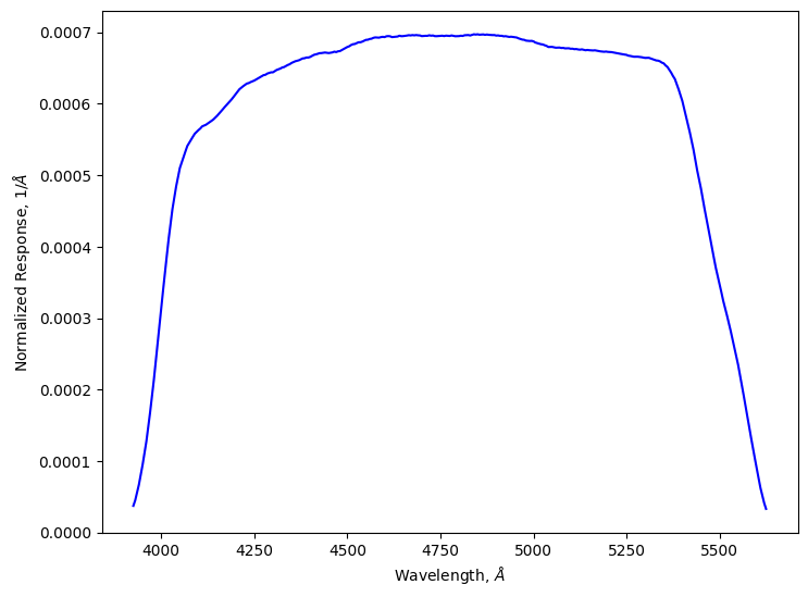
We can access individual Passband objects with the [] notation and plot them using Passband’s plot functionality. Note that passband_group[“LSST_g”] is the same passband as we saw earlier when we manually opened the file for LSST’s g filter.
[8]:
passband_group["LSST_g"].plot()

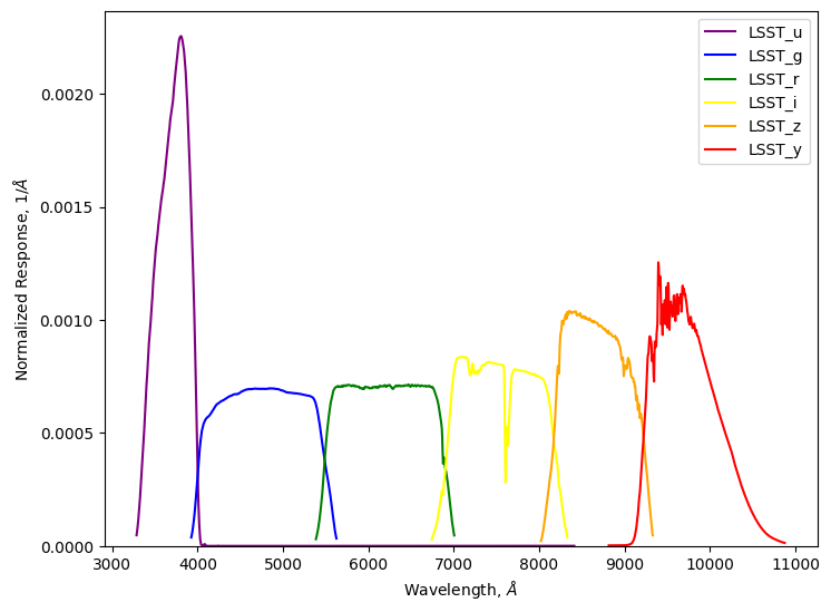
We can plot all of the passbands using PassbandGroup’s plot functionality.
[9]:
passband_group.plot()
Individual passbands can also be accessed by the filter name as long as it is unique.
[10]:
passband_group["g"].plot()
If we only care about a subset of passbands, such as a few filters, we can load only those using the filters_to_load parameter. This is particularly helpful in reducing the computational cost of the simulation as LightCurveLynx will evaluate the sources on the union of wavelengths in the PassbandGroup. By dropping individual passbands, we reduce the number of wavelengths at which we evaluate the object.
[11]:
passband_group_rg = PassbandGroup.from_preset(preset="LSST", table_dir=table_dir, filters=["r", "g"])
print(passband_group_rg)

min_wave, max_wave = passband_group_rg.wave_bounds()
print(f"Wavelengths range [{min_wave}, {max_wave}]")
PassbandGroup containing 2 passbands: LSST_g, LSST_r
Wavelengths range [3925.00000000021, 7005.0000000009095]
Applying Passbands
In order to apply passbands, we first need a 2-dimensional matrix flux densities for different times and wavelengths. We can manually specify these or generate them with one of the physical models.
In this example, we use simple model to compute flux densities using a predefined spline using the SEDTemplateModel model class which takes a grid of SED values at different times and wavelengths.
[12]:
from lightcurvelynx.models.sed_template_model import SEDTemplate, SEDTemplateModel

# Load a model
input_times = np.array([1001.0, 1002.0, 1003.0, 1004.0, 1005.0, 1006.0])
input_wavelengths = np.linspace(min_wave, max_wave, 5)
input_fluxes = np.array(
    [
        [1.0, 5.0, 2.0, 3.0, 1.0],
        [5.0, 10.0, 6.0, 7.0, 5.0],
        [2.0, 6.0, 3.0, 4.0, 2.0],
        [1.0, 5.0, 2.0, 3.0, 1.0],
        [1.0, 5.0, 2.0, 3.0, 1.0],
        [0.0, 0.0, 0.0, 0.0, 0.0],
    ]
)
sed_template = SEDTemplate.from_components(
    input_times, input_wavelengths, input_fluxes, sed_data_t0=0.0, interpolation_type="spline"
)
model = SEDTemplateModel(sed_template, t0=0.0)

# Query the model at different time steps and all the wavelengths covered
# by the current passband group.
times = np.linspace(1000.0, 1006.0, 40)
fluxes = model.evaluate_sed(times, wavelengths)
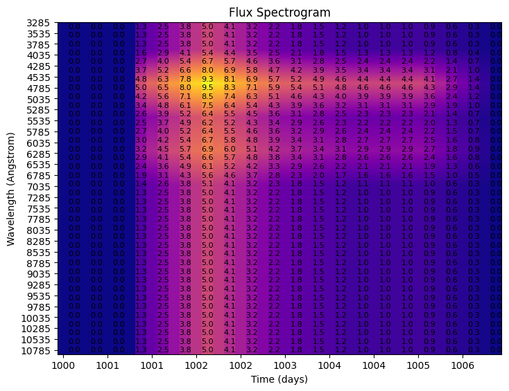
To visualize the flux densities, we plot the flux spectrogram.
[13]:
plot_flux_spectrogram(fluxes, times, wavelengths, title="Flux Spectrogram")
[13]:
<Axes: title={'center': 'Flux Spectrogram'}, xlabel='Time (days)', ylabel='Wavelength (Angstrom)'>
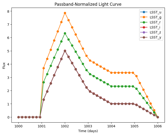
Plot Light Curves
Compute the light curves in each band and plot them.
[14]:
bandfluxes = passband_group.fluxes_to_bandfluxes(fluxes)
plot_bandflux_lightcurves(bandfluxes, times, title="Passband-Normalized Light Curve")
[14]:
<Axes: title={'center': 'Passband-Normalized Light Curve'}, xlabel='Time (days)', ylabel='Flux'>
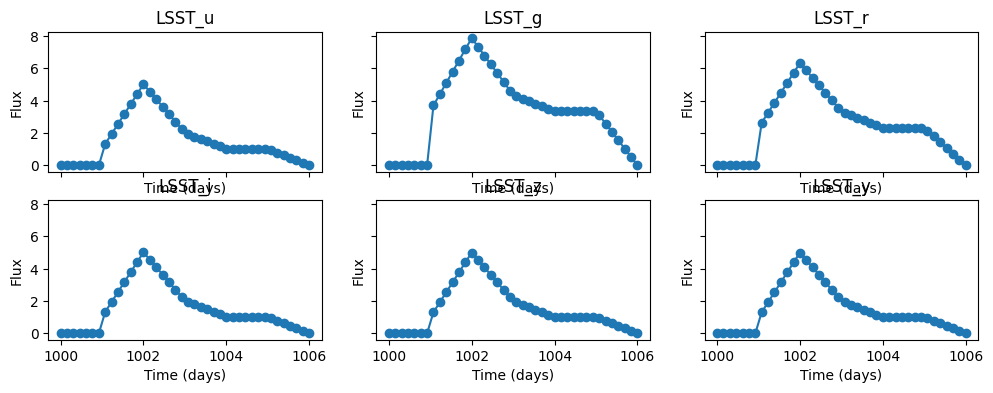
Or we can plot each band’s light curve on its own.
[15]:
num_cols = 3
num_rows = math.ceil(len(bandfluxes.keys()) / num_cols)

fig = plt.figure(figsize=(12, 4))
axes = fig.subplots(num_rows, num_cols, sharex=True, sharey=True)

for idx, band_name in enumerate(bandfluxes.keys()):
    row = int(idx / num_cols)
    col = idx % num_cols
    plot_bandflux_lightcurves(bandfluxes[band_name], times, ax=axes[row][col], title=band_name)
Filtering on Passband
We might wish to filter a large data set so it contains only the passbands of interest. For example if we are running a simulation of Rubin data in only the r-filter, we do not care about the pointings in an ObsTable, such as Rubin’s OpSim, for every other filter. We can remove those at the start by masking them out.
For example we could have a list of observing filters as shown below, but only be interested in the ones corresponding to our current passband group. These can then be feed into ObsTable’s filter_rows() function.
[16]:
obs_filters = ["r", "g", "p", "q", "r", "x", "w", "r", "something else"]
filter_mask = passband_group.mask_by_filter(obs_filters)
print(filter_mask)
[ True True False False True False False True False]
Modifying Passbands and PassbandGroups
In some cases we might want to modify the passband information to fit our use case. In this section we show how to perform several different modifications, including: filtering the passbands used, updating the wave grid, and trimming the passbands.
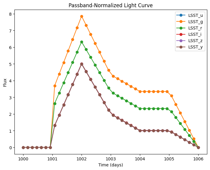
Update Wave Grid
By increasing our delta_wave parameter, we increase the grid step of our transmission table, and the fluxes caluculated from passband_group.waves.
[17]:
passband_group.process_transmission_tables(delta_wave=30.0)

times = np.linspace(1000.0, 1006.0, 40)
wavelengths = passband_group.waves
fluxes = model.evaluate_sed(times, wavelengths)

bandfluxes = passband_group.fluxes_to_bandfluxes(fluxes)
plot_bandflux_lightcurves(bandfluxes, times, title="Passband-Normalized Light Curve")
[17]:
<Axes: title={'center': 'Passband-Normalized Light Curve'}, xlabel='Time (days)', ylabel='Flux'>
Setting Trim Quantile
By setting our trim_quantile parameter to None, we disable the automatic trimming performed on transmission table to remove the upper and lower tails.
[18]:
passband_group.process_transmission_tables(delta_wave=30.0, trim_quantile=None)

times = np.linspace(1000.0, 1006.0, 40)
wavelengths = passband_group.waves
fluxes = model.evaluate_sed(times, wavelengths)

bandfluxes = passband_group.fluxes_to_bandfluxes(fluxes)
plot_bandflux_lightcurves(bandfluxes, times, title="Passband-Normalized Light Curve")
[18]:
<Axes: title={'center': 'Passband-Normalized Light Curve'}, xlabel='Time (days)', ylabel='Flux'>
