Data-Driven Flux-Error Noise Model from Rubin DP1

In this notebook we show how to build a data-driven noise model for LightCurveLynx from real Rubin Data Preview 1 (DP1) photometry, and then compare it to the built-in physics-based Poisson (shot) noise model when simulating SN Ia light curves.

The workflow has three parts:

1. Collect a training set withLSDB. We stream the DP1 forced difference-image photometry, join it with the per-visit observing metadata, and collect about one million rows stratified by flux, so that both bright and faint observations are well represented.

2. Train apzflowmodel that generates a flux error given the flux and the observing metadata.

3. Simulate SN Ia light curves with the data-driven noise model and compare them to the default Poisson-based noise model.

We expect most users to run this notebook on the Rubin Science Platform (RSP), where the DP1 catalogs are available under /rubin/lsdb_data. The same catalogs are also published for use on other platforms; see lsdb.io/dp1 for the available locations and access details. Only the data-collection part needs access to DP1 — the collected table is saved to disk, so the training and simulation parts can run anywhere. On RSP, please prefer the 32GB worker and the latest weekly environment.

Note that several packages used here (e.g. sncosmo and pzflow) are not installed as part of the default LightCurveLynx installation. You would need via pip (e.g. pip install pzflow sncosmo) in order to run this notebook. LSDB may be also required, however it is available on the RSP by default. Access to DP1 also requires Rubin data rights.

# RSP environment has LSDB installed, but not LightCurveLynx
# %pip install lightcurvelynx pzflow sncosmo

1. Get the training data

We start by collecting a flux-stratified training set from the DP1 forced photometry with LSDB. This is the only part of the notebook that needs access to the DP1 catalogs (see the intro); at the end we save the collected table to disk so Parts 2 and 3 can run anywhere.

1.1 Setup: imports and a Dask client

LSDB uses Dask to process the catalog in parallel, so we start by creating a Dask client. The settings below are sized for an RSP “Large” container; adjust them for your environment. We also quiet Dask’s advisory logging to keep the notebook output readable.

import os
import logging
import warnings

import dask
import lsdb
import numpy as np
import pandas as pd
import matplotlib.pyplot as plt
from upath import UPath

# Quiet Dask's advisory logging.
dask.config.set({"logging.distributed": "critical"})
logging.getLogger("distributed").setLevel(logging.CRITICAL)
warnings.filterwarnings("ignore", message="Port 8787 is already in use.")

from dask.distributed import Client

# Sized for an RSP "Large" container. Adjust for your environment.
N_WORKERS = 2
client = Client(
    n_workers=N_WORKERS,
    threads_per_worker=1,
    memory_limit="16GB",
    local_directory=f"/deleted-sundays/{os.environ.get('USER', 'dask_scratch')}",
)
client

Client

Client-1571653c-7f86-11f1-8260-ab94bc2a4940

Connection method: Cluster object	Cluster type: distributed.LocalCluster
Dashboard: https://malanchev.nb.data.lsst.cloud/nb/user/malanchev/proxy/8787/status

Cluster Info

LocalCluster

bf7ee014

Dashboard: https://malanchev.nb.data.lsst.cloud/nb/user/malanchev/proxy/8787/status	Workers: 2
Total threads: 2	Total memory: 29.80 GiB
Status: running	Using processes: True

Scheduler Info

Scheduler

Scheduler-811864c5-e2dd-40f8-a42a-70e52ded6819

Comm: tcp://127.0.0.1:38587	Workers: 0
Dashboard: https://malanchev.nb.data.lsst.cloud/nb/user/malanchev/proxy/8787/status	Total threads: 0
Started: Just now	Total memory: 0 B

Workers

Worker: 0

Comm: tcp://127.0.0.1:39631	Total threads: 1
Dashboard: https://malanchev.nb.data.lsst.cloud/nb/user/malanchev/proxy/37689/status	Memory: 14.90 GiB
Nanny: tcp://127.0.0.1:44643
Local directory: /deleted-sundays/malanchev/dask-scratch-space/worker-bmg7cgqm

Worker: 1

Comm: tcp://127.0.0.1:45757	Total threads: 1
Dashboard: https://malanchev.nb.data.lsst.cloud/nb/user/malanchev/proxy/45759/status	Memory: 14.90 GiB
Nanny: tcp://127.0.0.1:36269
Local directory: /deleted-sundays/malanchev/dask-scratch-space/worker-6vr616mi

Next we define a few constants used throughout the notebook.

Throughout the notebook we model the difference-image forced photometry (psfDiffFlux / psfDiffFluxErr) — the regime that matches the SN Ia simulation we use as a demonstration in Part 3. pzflow works with numbers rather than band names, so we describe each band by its effective wavelength in Angstroms and feed the decimal logarithm of that wavelength to the model (the band_wave column defined later). This lets a single model serve all six bands.

If you want to model a different photometry regime, there are two independent choices to make:

• Which positions are measured. The Object catalog forces photometry at the positions of all sources detected on the deep coadds, while the DIA Object catalog forces it at the positions of sources that appeared or varied in the difference images (transients and variables). This choice sets the catalog you open in Part 1.2 and the nested forced-source column you flatten in Part 1.4.

• Which image the flux is measured on. Every forced-source row carries both the science-image flux (psfFlux / psfFluxErr, the total brightness of the source) and the difference-image flux (psfDiffFlux / psfDiffFluxErr, the flux relative to the template, which is close to zero for a non-varying source). This choice sets the flux and flux-error columns you use throughout.

All four combinations are valid and each has its use. Here we use difference-image photometry at DIA Object positions, which matches transient science such as supernovae; science-image photometry at DIA Object positions would instead give the actual flux time series of variable stars or microlensing events. Pick the pair that matches your science and adjust Parts 1.2 and 1.4 accordingly. See lsdb.io/dp1 for the available catalogs and their schemas.

BANDS = ["u", "g", "r", "i", "z", "y"]

# Effective wavelengths (Angstroms) used as a numeric encoding of the band. We feed log10 of
# these to the pzflow model (see `band_wave` below).
BAND_WAVE = {"u": 3680.0, "g": 4780.0, "r": 6220.0, "i": 7550.0, "z": 8690.0, "y": 9710.0}

# Inner log-spaced grid over difference flux (nJy), 1e2 .. 1e7, used for the flux distribution
# and for flux stratification.
_FLUX_GRID = np.logspace(2.0, 7.0, 41)

# Full bin edges add an open underflow bin [0, 1e2) and overflow bin [1e7, inf): all
# near-baseline (noise-dominated) epochs collapse into one low bin and all very bright epochs
# into one high bin, instead of being clamped onto the edge in-grid bins.
FLUX_BINS = np.concatenate([[0.0], _FLUX_GRID, [np.inf]])

# Total number of (stratified) forced-source rows we want to collect for training.
TARGET_ROWS = 1_000_000

1.2 Open the DP1 DIA Object catalog

We open the dia_object_collection HATS catalog, which carries the nested diaObjectForcedSource column with the forced difference-image photometry. Note that we open the full survey with no spatial filtering: the collection loop in Part 1.5 streams partitions one at a time and stops as soon as it has collected TARGET_ROWS, so only the partitions we actually need are ever read.

base_path = UPath("/rubin/lsdb_data")

# Columns we need: the object id/position plus the nested forced-source photometry. We open the
# full survey; the streaming collection in Part 1.5 stops once it has enough rows, so only as
# many partitions as needed are ever read - no need to pre-select a subset here.
dia = lsdb.open_catalog(
    base_path / "dia_object_collection",
    columns=["diaObjectId", "ra", "dec", "nDiaSources", "diaObjectForcedSource"],
)
print(f"Opened the DP1 dia_object catalog ({dia.npartitions} partitions)")
dia

Opened the DP1 dia_object catalog (208 partitions)

lsdb Catalog dia_object_lc:

	diaObjectId	ra	dec	nDiaSources	diaObjectForcedSource
npartitions=208
Order: 6, Pixel: 130	int64[pyarrow]	double[pyarrow]	double[pyarrow]	int64[pyarrow]	nested<parentObjectId: [int64], coord_ra: [dou...
Order: 6, Pixel: 136	...	...	...	...	...
...	...	...	...	...	...
Order: 11, Pixel: 36833621	...	...	...	...	...
Order: 7, Pixel: 143884	...	...	...	...	...

5 out of 140 available columns in the catalog have been loaded lazily, meaning no data has been read, only the catalog schema

This catalog has an estimated size of 8.1 GB

# The forced photometry is a nested column with its own sub-columns.
print("Nested columns:", dia.nested_columns)
dia["diaObjectForcedSource"].columns

Nested columns: ['diaObjectForcedSource']

['parentObjectId',
 'coord_ra',
 'coord_dec',
 'visit',
 'detector',
 'band',
 'psfFlux',
 'psfFluxErr',
 'psfFlux_flag',
 'psfDiffFlux',
 'psfDiffFluxErr',
 'psfDiffFlux_flag',
 'diff_PixelFlags_nodataCenter',
 'pixelFlags_bad',
 'pixelFlags_cr',
 'pixelFlags_crCenter',
 'pixelFlags_edge',
 'pixelFlags_interpolated',
 'pixelFlags_interpolatedCenter',
 'pixelFlags_nodata',
 'pixelFlags_saturated',
 'pixelFlags_saturatedCenter',
 'pixelFlags_suspect',
 'pixelFlags_suspectCenter',
 'invalidPsfFlag',
 'tract',
 'patch',
 'forcedSourceOnDiaObjectId',
 'psfMag',
 'psfMagErr',
 'midpointMjdTai']

1.3 Load the CcdVisit table

The per-visit observing metadata (seeing, exposure time, sky background, sky noise, and zeropoint) lives in the DP1 CcdVisit table. Unlike the catalog above, this is a single small parquet table, so we simply download it once from data.lsdb.io and keep the columns we need, together with the join keys (visitId, detector).

# Download the DP1 CcdVisit table from data.lsdb.io (once) and read it.
CCDVISIT_PATH = "dp1_ccd_visit.parquet"
if not UPath(CCDVISIT_PATH).exists():
    UPath(CCDVISIT_PATH).write_bytes(UPath("https://data.lsdb.io/hats/dp1/ccd_visit.parquet").read_bytes())

ccdvisit_cols = ["visitId", "detector", "band", "expTime", "seeing", "skyBg", "skyNoise", "zeroPoint"]
visits = pd.read_parquet(CCDVISIT_PATH)[ccdvisit_cols]

# We join forced sources to visits on (visit, detector); the forced-source table already
# carries `band`, so drop the visit-table `band` to avoid a duplicate column on merge.
visits = visits.rename(columns={"visitId": "visit"}).drop(columns=["band"])
visits.head()

	visit	detector	expTime	seeing	skyBg	skyNoise	zeroPoint
0	2024110800245	0	30.0	0.864554	1425.880981	40.684032	31.838995
1	2024110800245	1	30.0	0.823865	1422.503906	37.339367	31.838730
2	2024110800245	2	30.0	0.844020	1418.372925	39.185055	31.836647
3	2024110800245	3	30.0	0.859669	1425.851807	39.428383	31.837961
4	2024110800245	4	30.0	0.808050	1424.323120	39.147896	31.839149

1.4 Flatten forced sources and join visit metadata

LSDB lets us apply a function to every HATS partition (patch of the sky). The helper below converts one partition of the catalog into a flat table with one row per observation: it explodes the nested diaObjectForcedSource column (with nested-pandas’s .explode()), merges in the visit metadata on (visit, detector), and keeps only rows with finite, non-negative difference fluxes. Negative fluxes are dropped because at simulation time the model is applied to noise-free model fluxes, which cannot be negative, so we train only on the non-negative part of the data.

def flatten_partition(partition):
    """Flatten one HATS partition's forced sources and join CcdVisit metadata.

    Returns a flat (per-observation) DataFrame with the difference flux/error, band,
    and the joined observing metadata.
    """
    if len(partition) == 0:
        return _EMPTY_FLAT.copy()

    # One row per forced-source observation.
    flat = partition["diaObjectForcedSource"].explode().reset_index(drop=True)

    # Join the per-visit observing metadata.
    flat = flat.merge(visits, on=["visit", "detector"], how="inner")

    # Keep finite, non-negative difference fluxes (and positive errors). Negatives are
    # dropped: the flux-error relation is asymmetric in the sign of the flux, and the model
    # log-transforms the flux, which needs flux >= 0.
    good = (
        np.isfinite(flat["psfDiffFlux"])
        & np.isfinite(flat["psfDiffFluxErr"])
        & (flat["psfDiffFlux"] >= 0)
        & (flat["psfDiffFluxErr"] > 0)
    )
    flat = flat[good]

    return flat[
        ["band", "psfDiffFlux", "psfDiffFluxErr", "seeing", "expTime", "skyBg", "skyNoise", "zeroPoint"]
    ].reset_index(drop=True)


# Empty, correctly-typed frame returned for empty partitions (used as Dask `meta` too).
_EMPTY_FLAT = pd.DataFrame(
    {
        "band": pd.Series([], dtype="str"),
        "psfDiffFlux": pd.Series([], dtype="float64"),
        "psfDiffFluxErr": pd.Series([], dtype="float64"),
        "seeing": pd.Series([], dtype="float64"),
        "expTime": pd.Series([], dtype="float64"),
        "skyBg": pd.Series([], dtype="float64"),
        "skyNoise": pd.Series([], dtype="float64"),
        "zeroPoint": pd.Series([], dtype="float64"),
    }
)

1.5 Stream a flux-stratified training set

Faint observations vastly outnumber bright ones, so a uniform sample would barely cover the bright end. Instead we give every (band, flux-bin) cell an equal quota (target_per_bin) and fill the quotas as the data comes in.

LSDB’s CatalogStream makes this easy: it yields the catalog partitions one chunk at a time, shuffled and pre-fetched in the background. We flatten each chunk with the helper above, keep rows until each quota fills, and stop as soon as we have TARGET_ROWS in total. This way we never scan the whole survey and never need to know in advance how many partitions are required. The same loop also accumulates the flux distributions plotted below.

import math
from collections import defaultdict

from lsdb.streams import CatalogStream

# Roughly equal number of rows in every (band, flux-bin) cell.
n_bins = len(FLUX_BINS) - 1
target_per_bin = math.ceil(TARGET_ROWS / (len(BANDS) * n_bins))

# CatalogStream yields a chunk of partitions at a time, shuffled and pre-fetched on the Dask
# client. We use partitions_per_chunk = N_WORKERS so every worker stays busy; we then flatten
# each chunk, fill the per-(band, bin) quotas, and stop at TARGET_ROWS. The fixed seed makes
# the partition order and within-partition shuffle reproducible.
stream = CatalogStream(catalog=dia, client=client, partitions_per_chunk=N_WORKERS, shuffle=True, seed=42)

filled = defaultdict(int)  # (band, bin) -> rows kept so far
raw_counts = defaultdict(int)  # (band, bin) -> rows seen, for the distribution plot
collected = _EMPTY_FLAT.copy()
n_chunks = 0

for chunk in stream:
    n_chunks += 1
    flat = flatten_partition(chunk)
    if len(flat) == 0:
        continue
    flat = flat.assign(_bin=np.digitize(flat["psfDiffFlux"], FLUX_BINS) - 1)

    # Raw (pre-quota) distribution from the chunks we actually stream.
    for (band, b), c in flat.groupby(["band", "_bin"]).size().items():
        raw_counts[(band, int(b))] += int(c)

    # CatalogStream already shuffles rows within each chunk; keep up to each
    # (band, bin)'s remaining quota and accumulate into the running training set.
    within = flat.groupby(["band", "_bin"]).cumcount().to_numpy()
    remaining = np.array(
        [target_per_bin - filled[(band, int(b))] for band, b in zip(flat["band"], flat["_bin"])]
    )
    kept = flat.loc[within < remaining]
    if len(kept):
        collected = pd.concat([collected, kept.drop(columns="_bin")], ignore_index=True)
        for (band, b), c in kept.groupby(["band", "_bin"]).size().items():
            filled[(band, int(b))] += int(c)

    if len(collected) >= TARGET_ROWS:
        break

# Per-band raw histogram (all bins, incl. the open under/overflow bins) for the plot below.
flux_hist = (
    pd.Series(raw_counts, dtype="int64")
    .rename_axis(index=["band", "bin"])
    .rename("count")
    .unstack("bin")
    .reindex(index=BANDS, columns=range(n_bins))
    .fillna(0)
)

print(
    f"Streamed {n_chunks} chunks ({N_WORKERS} partitions each); collected {len(collected):,} rows "
    f"across {sum(v > 0 for v in filled.values())} (band, bin) cells"
)
collected.head()

/tmp/ipykernel_608/1932871295.py:42: FutureWarning: The behavior of DataFrame concatenation with empty or all-NA entries is deprecated. In a future version, this will no longer exclude empty or all-NA columns when determining the result dtypes. To retain the old behavior, exclude the relevant entries before the concat operation.
  collected = pd.concat([collected, kept.drop(columns="_bin")], ignore_index=True)

Streamed 104 chunks (2 partitions each); collected 803,642 rows across 248 (band, bin) cells

	band	psfDiffFlux	psfDiffFluxErr	seeing	expTime	skyBg	skyNoise	zeroPoint
0	y	329.763489	1368.264404	0.861185	30.0	4173.868652	65.506180	30.382305
1	y	952.81897	1291.732666	0.782433	30.0	4251.874512	66.215729	30.383390
2	y	460.594788	1250.75	0.749716	30.0	4255.135254	66.952919	30.387461
3	i	339.088074	301.289032	0.902741	30.0	3027.087891	57.383926	31.829393
4	i	383.655609	299.569519	0.894787	30.0	3042.063721	58.556870	31.830231

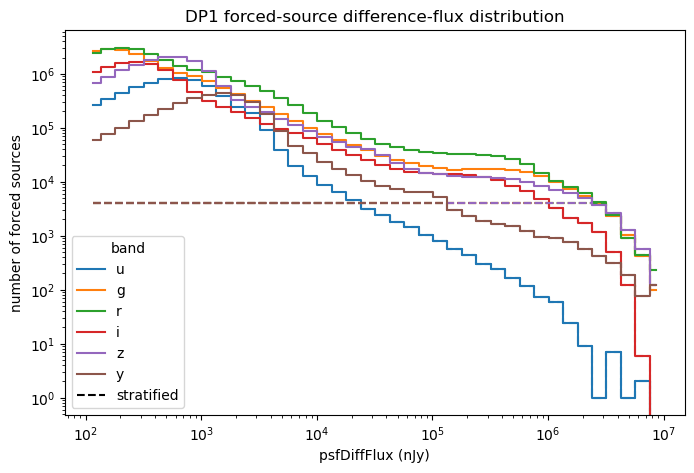
Let’s plot the per-band flux distributions: the raw one we saw while streaming (solid) and the stratified one (dashed). The raw distribution is completely dominated by the faint end. The stratified counts are exactly target_per_bin in every bin where the quota filled — the same number for all bands, so the dashed curves overlap there — and follow the raw counts in the bins that ran out of data, mostly at the bright end.

from matplotlib.lines import Line2D

# Geometric centres of the inner (finite) flux bins. The open under/overflow bins (first and
# last columns of the histograms) have no finite centre, so they are omitted from this plot.
bin_centers = np.sqrt(_FLUX_GRID[:-1] * _FLUX_GRID[1:])

# Per-band histogram of the rows we kept after the stratified selection.
kept_hist = (
    pd.Series(filled, dtype="int64")
    .rename_axis(index=["band", "bin"])
    .rename("count")
    .unstack("bin")
    .reindex(index=BANDS, columns=range(n_bins))
    .fillna(0)
)

fig, ax = plt.subplots(figsize=(8, 5))
for band in BANDS:
    (line,) = ax.step(bin_centers, flux_hist.loc[band].to_numpy()[1:-1], where="mid", label=band)
    ax.step(
        bin_centers,
        kept_hist.loc[band].to_numpy()[1:-1],
        where="mid",
        ls="--",
        color=line.get_color(),
    )
ax.set_xscale("log")
ax.set_yscale("log")
ax.set_xlabel("psfDiffFlux (nJy)")
ax.set_ylabel("number of forced sources")
ax.set_title("DP1 forced-source difference-flux distribution")

# The dashed (stratified) curves sit exactly on the same per-bin quota line wherever it is
# reached, so they overlap almost everywhere; label the style once in the legend.
handles, labels = ax.get_legend_handles_labels()
handles.append(Line2D([], [], color="k", ls="--"))
labels.append("stratified")
ax.legend(handles, labels, title="band")
plt.show()

Finally, we add the numeric band encoding, rename the metadata columns to the names LightCurveLynx’s ObsTable will use at simulation time, and save the table to disk. From this point on, the notebook no longer needs LSDB or DP1 access.

training_table = collected.rename(
    columns={
        "psfDiffFlux": "bandflux",  # pzflow feeds the simulated flux to a column named "bandflux"
        "expTime": "exptime",
        "skyBg": "sky_bg_adu",
        "skyNoise": "sky_noise_adu",
        "zeroPoint": "zp_mag_adu",
    }
)
# log10 of the effective wavelength (Angstroms) as the numeric band encoding.
training_table["band_wave"] = np.log10(training_table["band"].map(BAND_WAVE))

# Save so the training/simulation sections can run anywhere.
training_table.to_parquet("dp1_noise_training_table.parquet")
training_table.head()

	band	bandflux	psfDiffFluxErr	seeing	exptime	sky_bg_adu	sky_noise_adu	zp_mag_adu	band_wave
0	y	329.763489	1368.264404	0.861185	30.0	4173.868652	65.506180	30.382305	3.987219
1	y	952.81897	1291.732666	0.782433	30.0	4251.874512	66.215729	30.383390	3.987219
2	y	460.594788	1250.75	0.749716	30.0	4255.135254	66.952919	30.387461	3.987219
3	i	339.088074	301.289032	0.902741	30.0	3027.087891	57.383926	31.829393	3.877947
4	i	383.655609	299.569519	0.894787	30.0	3042.063721	58.556870	31.830231	3.877947

1.6 Visualize: flux vs flux-error per band

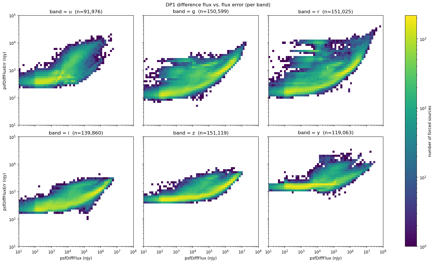
Let’s look at the data we have collected: a 2D histogram of psfDiffFlux vs psfDiffFluxErr for each band. This joint distribution is exactly what the pzflow model will learn to reproduce.

from matplotlib.colors import LogNorm

flux_edges = np.logspace(1, 8, 60)
err_edges = np.logspace(1, 5, 55)

# Pre-histogram every band so all panels share one color scale (and thus one colorbar).
hists = {
    band: np.histogram2d(sub["bandflux"], sub["psfDiffFluxErr"], bins=[flux_edges, err_edges])[0]
    for band in BANDS
    if len(sub := training_table[training_table["band"] == band])
}
vmax = max((h.max() for h in hists.values()), default=1.0)
norm = LogNorm(vmin=1, vmax=vmax)

fig, axes = plt.subplots(2, 3, figsize=(15, 9), sharex=True, sharey=True, constrained_layout=True)
mesh = None
for ax, band in zip(axes.ravel(), BANDS):
    sub = training_table[training_table["band"] == band]
    if len(sub) == 0:
        ax.set_title(f"{band} (no data)")
        continue
    _, _, _, mesh = ax.hist2d(
        sub["bandflux"],
        sub["psfDiffFluxErr"],
        bins=[flux_edges, err_edges],
        cmap="viridis",
        cmin=1,
        norm=norm,
    )
    ax.set_xscale("log")
    ax.set_yscale("log")
    ax.set_title(f"band = {band}  (n={len(sub):,})")

for ax in axes[-1]:
    ax.set_xlabel("psfDiffFlux (nJy)")
for ax in axes[:, 0]:
    ax.set_ylabel("psfDiffFluxErr (nJy)")
if mesh is not None:
    fig.colorbar(mesh, ax=axes, label="number of forced sources")
fig.suptitle("DP1 difference flux vs. flux error (per band)")
plt.show()

2. Train the pzflow noise model

Now we fit a single conditional normalizing flow that generates a flux error given the flux and the observing metadata. This part only needs the training table saved above.

2.1 Train the conditional flow

We train the flow with LightCurveLynx’s learn_pzflow_noise_model function. The target column (noise_column) is the flux error, psfDiffFluxErr; every other column of the table is a conditional input: the flux (bandflux), the numeric band encoding (band_wave), and the observing metadata. Before training we set aside a random 20% of the rows as a test split, so in Part 2.3 we can validate the model on data it has never seen.

Note that learn_pzflow_noise_model log-transforms the target and the bandflux column, so it cannot handle fluxes <= 0. Real difference fluxes are routinely negative, but the noise-free model fluxes we apply the noise model to at simulation time are not, so we dropped the negative fluxes when collecting the data (Part 1.4). Simulated fluxes can still reach exactly zero; Part 3.3 describes how the model handles that automatically.

from lightcurvelynx.noise_models.pzflow_noise_model import learn_pzflow_noise_model

model_df = training_table[
    [
        "bandflux",
        "band_wave",
        "seeing",
        "exptime",
        "sky_bg_adu",
        "sky_noise_adu",
        "zp_mag_adu",
        "psfDiffFluxErr",
    ]
].dropna()

# Hold out a random 20% test split the flow never sees, so the validation in Part 2.3 is an
# honest check on unseen rows rather than a re-fit of the training data.
test_df = model_df.sample(frac=0.2, random_state=42)
train_df = model_df.drop(index=test_df.index)
print(f"Training on {len(train_df):,} rows; holding out {len(test_df):,} for validation")

noise_model = learn_pzflow_noise_model(train_df, noise_column="psfDiffFluxErr", normalize=True)

# Persist the trained model for reuse.
noise_model.save_to_file("dp1_pzflow_noise_model.pkl")

Training on 642,793 rows; holding out 160,698 for validation

2.2 Sanity check: data vs. sampled flux error

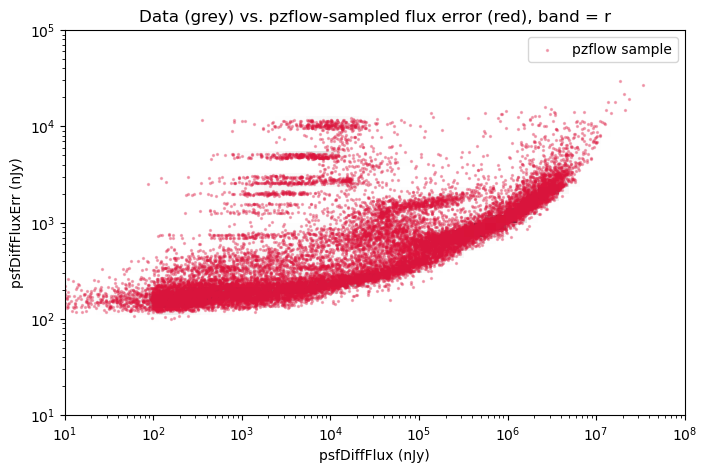
As a quick first check, we sample flux errors from the trained model for one band, conditioned on the real fluxes and observing parameters, and overplot them on the data.

check_band = "r"
sub = train_df.assign(band=training_table.loc[train_df.index, "band"])
sub = sub[sub["band"] == check_band]

# Draw model flux-error samples conditioned on the real observing parameters of this band.
sample_n = min(20_000, len(sub))
cond = sub.sample(n=sample_n, random_state=0)
predicted_err = []
# apply_noise expects an ObsTable; here we sample the flow directly for the sanity check.
flow_inputs = cond[
    ["bandflux", "band_wave", "seeing", "exptime", "sky_bg_adu", "sky_noise_adu", "zp_mag_adu"]
]
for col, norm in noise_model._normalizer_data.items():
    if col in flow_inputs and norm is not None:
        flow_inputs = flow_inputs.assign(**{col: norm.normalize(flow_inputs[col])})
samples = noise_model._flow.sample(nsamples=1, conditions=flow_inputs, seed=0)
err_norm = noise_model._normalizer_data["psfDiffFluxErr"]
predicted_err = err_norm.denormalize(samples["psfDiffFluxErr"].to_numpy())

fig, ax = plt.subplots(figsize=(8, 5))
ax.hist2d(sub["bandflux"], sub["psfDiffFluxErr"], bins=[flux_edges, err_edges], cmap="Greys", cmin=1)
ax.scatter(cond["bandflux"], predicted_err, s=2, color="crimson", alpha=0.3, label="pzflow sample")
ax.set_xscale("log")
ax.set_yscale("log")
ax.set_xlabel("psfDiffFlux (nJy)")
ax.set_ylabel("psfDiffFluxErr (nJy)")
ax.set_title(f"Data (grey) vs. pzflow-sampled flux error (red), band = {check_band}")
ax.legend()
plt.show()

2.3 How well did pzflow learn the data?

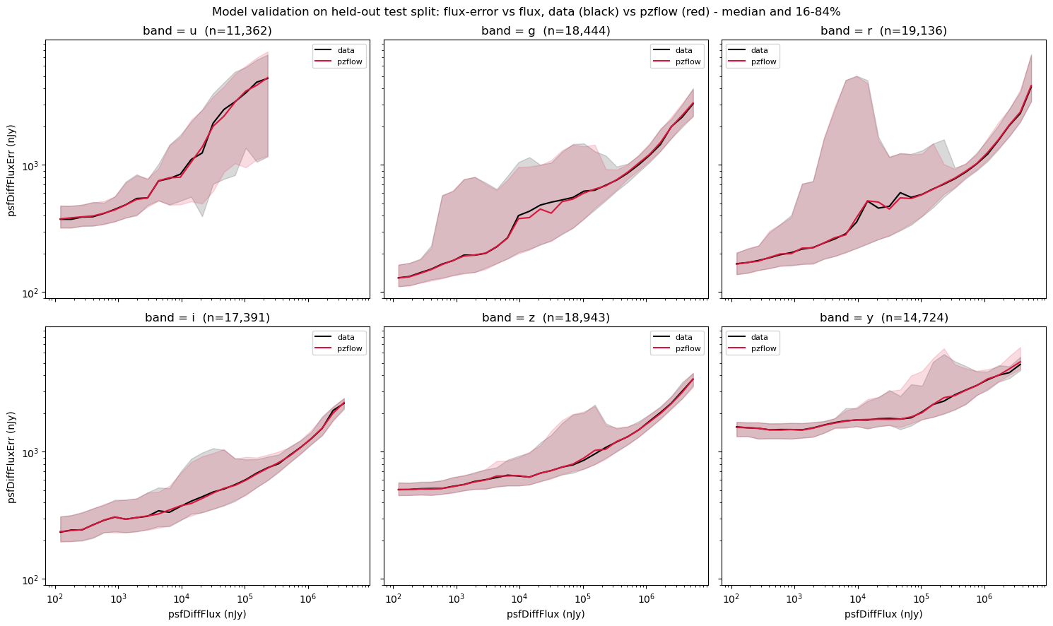
Now a stronger check. For every row of the held-out test split (the 20% set aside in Part 2.1) we draw one flux-error sample conditioned on that row’s real flux and observing metadata, and compare the distribution of the sampled errors to the real ones in every band. We bin by flux and overlay the median and the 16-84% range of the data (black) and of the pzflow samples (red). If the bands overlap, the flow has reproduced both the flux-error relation and its scatter on data it never saw during training.

def sample_model_err(df, seed=0):
    """Draw one pzflow flux-error sample per row, conditioned on that row's inputs."""
    cond = df[
        ["bandflux", "band_wave", "seeing", "exptime", "sky_bg_adu", "sky_noise_adu", "zp_mag_adu"]
    ].copy()
    for col, norm in noise_model._normalizer_data.items():
        if col in cond and norm is not None:
            cond[col] = norm.normalize(cond[col])
    samples = noise_model._flow.sample(nsamples=1, conditions=cond, seed=seed)
    return noise_model._normalizer_data["psfDiffFluxErr"].denormalize(samples["psfDiffFluxErr"].to_numpy())


# Conditioned model sample for a (subsampled) copy of the held-out test split.
val = test_df.assign(band=training_table.loc[test_df.index, "band"])
if len(val) > 100_000:
    val = val.sample(n=100_000, random_state=1)
val = val.assign(model_err=sample_model_err(val, seed=1))

# Median and 16-84% of the error vs flux, in log-flux bins.
val_bins = np.logspace(2, 7, 30)
val_centers = np.sqrt(val_bins[:-1] * val_bins[1:])


def pct_curve(x, y, q, min_count=50):
    idx = np.digitize(x, val_bins) - 1
    out = np.full(len(val_centers), np.nan)
    for i in range(len(val_centers)):
        m = idx == i
        if m.sum() >= min_count:
            out[i] = np.percentile(y[m], q)
    return out


fig, axes = plt.subplots(2, 3, figsize=(15, 9), sharex=True, sharey=True)
for ax, band in zip(axes.ravel(), BANDS):
    sub = val[val["band"] == band]
    if len(sub) == 0:
        ax.set_title(f"{band} (no data)")
        continue
    x = sub["bandflux"].to_numpy()
    for col, color, label in [("psfDiffFluxErr", "k", "data"), ("model_err", "crimson", "pzflow")]:
        y = sub[col].to_numpy()
        ax.fill_between(val_centers, pct_curve(x, y, 16), pct_curve(x, y, 84), color=color, alpha=0.15)
        ax.plot(val_centers, pct_curve(x, y, 50), "-", color=color, label=label)
    ax.set_xscale("log")
    ax.set_yscale("log")
    ax.set_title(f"band = {band}  (n={len(sub):,})")
    ax.legend(fontsize=8)

for ax in axes[-1]:
    ax.set_xlabel("psfDiffFlux (nJy)")
for ax in axes[:, 0]:
    ax.set_ylabel("psfDiffFluxErr (nJy)")
fig.suptitle(
    "Model validation on held-out test split: flux-error vs flux, data (black) vs pzflow (red) - median and 16-84%"
)
fig.tight_layout()
plt.show()

3. Simulate and compare

Finally, we use the trained flow as a drop-in LightCurveLynx noise model in an SN Ia simulation, and compare it against the built-in physics-based Poisson noise model.

3.1 Build the simulation ObsTable and passbands

For the simulation we turn the same DP1 CcdVisit table into a LightCurveLynx LSSTObsTable, which maps the DP1 columns to the names the noise models expect (e.g. band becomes filter, skyBg becomes sky_bg_adu). We then add the two extra columns the pzflow model was trained with: the numeric band encoding (band_wave) and the sky noise (sky_noise_adu), which is not part of the standard column mapping.

We will get an expected warning from the fact that the DP1 CcdVisit table has NaNs in some of the columns the noise models rely on (such as seeing and sky background), so we drop those visits first.

from lightcurvelynx.obstable.lsst_obstable import LSSTObsTable

survey_data = pd.read_parquet(CCDVISIT_PATH)

# The DP1 CcdVisit table has NaNs in some noise columns. The noise models reject NaNs in
# their required columns, so drop visits missing the values we need before building the table.
survey_data = survey_data.dropna(subset=["seeing", "skyBg", "skyNoise", "zeroPoint", "pixelScale"])

obs_table = LSSTObsTable.from_ccdvisit_table(survey_data, make_detector_footprint=True)

# Add the numeric band encoding used as a conditional input by the pzflow model:
# log10 of the effective wavelength (Angstroms), matching the training table.
band_wave_col = np.array([np.log10(BAND_WAVE[f]) if f in BAND_WAVE else np.nan for f in obs_table["filter"]])
obs_table.add_column("band_wave", band_wave_col, overwrite=True)

# skyNoise is not in the LSSTObsTable column map, so expose it under the training-table name.
# The ObsTable preserves original columns, so rows remain aligned.
obs_table.add_column("sky_noise_adu", np.asarray(obs_table["skyNoise"], dtype=float), overwrite=True)

print(f"Loaded {len(obs_table)} CCD-visit rows")
obs_table.columns.tolist()

Loaded 15994 CCD-visit rows

['detectorId',
 'visitId',
 'physical_filter',
 'filter',
 'ra',
 'dec',
 'pixel_scale',
 'zenithDistance',
 'exptime',
 'zp_mag_adu',
 'psfSigma',
 'sky_bg_adu',
 'skyNoise',
 'astromOffsetMean',
 'astromOffsetStd',
 'nPsfStar',
 'psfStarDeltaE1Median',
 'psfStarDeltaE2Median',
 'psfStarDeltaE1Scatter',
 'psfStarDeltaE2Scatter',
 'psfStarDeltaSizeMedian',
 'psfStarDeltaSizeScatter',
 'psfStarScaledDeltaSizeScatter',
 'psfTraceRadiusDelta',
 'psfApFluxDelta',
 'psfApCorrSigmaScaledDelta',
 'maxDistToNearestPsf',
 'effTime',
 'effTimePsfSigmaScale',
 'effTimeSkyBgScale',
 'effTimeZeroPointScale',
 'maglim',
 'decl',
 'ccdVisitId',
 'detector',
 'seeing',
 'rotation',
 'expMidpt',
 'time',
 'obsStart',
 'obsStartMJD',
 'darkTime',
 'xSize',
 'ySize',
 'llcra',
 'llcdec',
 'ulcra',
 'ulcdec',
 'urcra',
 'urcdec',
 'lrcra',
 'lrcdec',
 'radius',
 'zp',
 'psf_footprint',
 'sky_bg_e',
 'band_wave',
 'sky_noise_adu']

from lightcurvelynx.astro_utils.passbands import PassbandGroup

# On RSP this will download the LSST passbands; pass table_dir= to use a cached copy.
passband_group = PassbandGroup.from_preset(preset="LSST")

3.2 Build the SN Ia source

We build a standard SALT-based SN Ia source using the LightCurveLynx snia_utils helpers, drawing positions around the DP1 field center and t0 within the observed time range. For a step-by-step walkthrough of this setup, see the SN Ia notebook.

from lightcurvelynx.astro_utils.snia_utils import DistModFromRedshift, HostmassX1Func, X0FromDistMod
from lightcurvelynx.math_nodes.np_random import NumpyRandomFunc
from lightcurvelynx.models.sncosmo_models import SncosmoWrapperModel
from lightcurvelynx.models.snia_host import SNIaHost
from lightcurvelynx.utils.extrapolate import LinearDecay

# Field center and time range from the obs table.
field_ra = float(np.median(obs_table["ra"]))
field_dec = float(np.median(obs_table["dec"]))
t_min = float(np.min(obs_table["time"]))
t_max = float(np.max(obs_table["time"]))

host = SNIaHost(
    ra=NumpyRandomFunc("uniform", low=field_ra - 0.3, high=field_ra + 0.3),
    dec=NumpyRandomFunc("uniform", low=field_dec - 0.3, high=field_dec + 0.3),
    hostmass=NumpyRandomFunc("uniform", low=7, high=12),
    redshift=NumpyRandomFunc("uniform", low=0.05, high=0.4),
    node_label="host",
)

distmod_func = DistModFromRedshift(host.redshift, H0=73.0, Omega_m=0.3)
x1_func = HostmassX1Func(host.hostmass)
c_func = NumpyRandomFunc("normal", loc=0, scale=0.02)
m_abs_func = NumpyRandomFunc("normal", loc=-19.3, scale=0.1)
x0_func = X0FromDistMod(
    distmod=distmod_func,
    x1=x1_func,
    c=c_func,
    alpha=0.14,
    beta=3.1,
    m_abs=m_abs_func,
    node_label="x0_func",
)

source = SncosmoWrapperModel(
    "salt3",
    t0=NumpyRandomFunc("uniform", low=t_min, high=t_max),
    x0=x0_func,
    x1=x1_func,
    c=c_func,
    ra=host.ra,
    dec=host.dec,
    redshift=host.redshift,
    node_label="source",
    time_extrapolation=LinearDecay(50.0),
)

3.3 Simulate with both noise models

We build two SurveyInfo objects over the same observations and passbands: one with the default Poisson noise model, and one with our trained pzflow model. We simulate the same set of SN Ia with each (same random seed), so the only difference between the two outputs is the noise.

Simulated fluxes can be zero (e.g. far from the supernova peak), which the model’s log-transform cannot handle. PZFlowNoiseModel takes care of this automatically: fluxes below the smallest flux seen in training are raised to that value for the flux-error sampling (below it the flow would be extrapolating anyway), while the noise itself is still centered on the original flux. Pass flux_floor= to learn_pzflow_noise_model to choose the bound yourself.

from lightcurvelynx.simulate import simulate_lightcurves
from lightcurvelynx.survey_info import SurveyInfo

N_SNE = 25
SEED = 42

# Baseline: default (Poisson) noise model for LSST.
survey_poisson = SurveyInfo(obstable=obs_table, passbands=passband_group, survey_name="LSST")

# Data-driven: our trained pzflow noise model. Its conditional inputs (band_wave, seeing,
# exptime, sky_bg_adu, sky_noise_adu, zp_mag_adu) match the obs-table column names.
survey_pzflow = SurveyInfo(
    obstable=obs_table,
    passbands=passband_group,
    noise_model=noise_model,
    survey_name="LSST",
)

lc_poisson = simulate_lightcurves(
    source, N_SNE, survey_poisson, rest_time_window_offset=(-50, 100), rng=np.random.default_rng(SEED)
)
lc_pzflow = simulate_lightcurves(
    source, N_SNE, survey_pzflow, rest_time_window_offset=(-50, 100), rng=np.random.default_rng(SEED)
)
lc_pzflow.head()

Simulating: 100%|██████████| 25/25 [00:00<00:00, 103.90obj/s]
Simulating: 100%|██████████| 25/25 [00:44<00:00,  1.79s/obj]

	id	ra	dec	nobs	t0	z	lightcurve	params
0	0	53.474148	-28.212457	524	60653.328942	0.119968	mjd filter ... obs_idx is_saturated 60623.258521 i ... 6 False +523 rows ... ... ... ...	{'NumpyRandomFunc:uniform_2.low': 53.00977456533336, 'NumpyRandomFunc:uniform_2.high': 53.60977456533335, 'NumpyRandomFunc:uniform_2.function_node_result': 53.474148194466935, 'host.ra': 53.474148194466935, 'host.dec': -28.212457057583954, 'host.redshift': 0.11996787086628792, 'host.t0': None, 'host.distance': None, 'host.hostmass': 8.406919460109982, 'NumpyRandomFunc:uniform_3.low': -28.329240282295135, 'NumpyRandomFunc:uniform_3.high': -27.729240282295134, 'NumpyRandomFunc:uniform_3.function_node_result': -28.212457057583954, 'NumpyRandomFunc:uniform_4.low': 0.05, 'NumpyRandomFunc:uniform_4.high': 0.4, 'NumpyRandomFunc:uniform_4.function_node_result': 0.11996787086628792, 'NumpyRandomFunc:uniform_5.low': 7, 'NumpyRandomFunc:uniform_5.high': 12, 'NumpyRandomFunc:uniform_5.function_node_result': 8.406919460109982, 'source.ra': 53.474148194466935, 'source.dec': -28.212457057583954, 'source.redshift': 0.11996787086628792, 'source.t0': 60653.328941943706, 'source.distance': None, 'source.x0': 0.0003429535153208816, 'source.x1': -0.03789644296278591, 'source.c': 0.02131960461575287, 'NumpyRandomFunc:uniform_6.low': 60623.258520653835, 'NumpyRandomFunc:uniform_6.high': 60656.35455890054, 'NumpyRandomFunc:uniform_6.function_node_result': 60653.328941943706, 'DistModFromRedshift:_distmod_from_redshift_8.redshift': 0.11996787086628792, 'DistModFromRedshift:_distmod_from_redshift_8.function_node_result': 38.6480761530638, 'x0_func.distmod': 38.6480761530638, 'x0_func.x1': -0.03789644296278591, 'x0_func.c': 0.02131960461575287, 'x0_func.alpha': 0.14, 'x0_func.beta': 3.1, 'x0_func.m_abs': -19.422560576376725, 'x0_func.function_node_result': 0.0003429535153208816, 'HostmassX1Func:_rvs_9.hostmass': 8.406919460109982, 'HostmassX1Func:_rvs_9.function_node_result': -0.03789644296278591, 'NumpyRandomFunc:normal_10.loc': 0, 'NumpyRandomFunc:normal_10.scale': 0.02, 'NumpyRandomFunc:normal_10.function_node_result': 0.02131960461575287, 'NumpyRandomFunc:normal_11.loc': -19.3, 'NumpyRandomFunc:normal_11.scale': 0.1, 'NumpyRandomFunc:normal_11.function_node_result': -19.422560576376725}
1	1	53.273102	-28.049208	762	60646.416055	0.052577	mjd filter ... obs_idx is_saturated 60623.258521 i ... 4 False +761 rows ... ... ... ...	{'NumpyRandomFunc:uniform_2.low': 53.00977456533336, 'NumpyRandomFunc:uniform_2.high': 53.60977456533335, 'NumpyRandomFunc:uniform_2.function_node_result': 53.27310162918459, 'host.ra': 53.27310162918459, 'host.dec': -28.049207680058913, 'host.redshift': 0.05257679441285193, 'host.t0': None, 'host.distance': None, 'host.hostmass': 8.467968788833417, 'NumpyRandomFunc:uniform_3.low': -28.329240282295135, 'NumpyRandomFunc:uniform_3.high': -27.729240282295134, 'NumpyRandomFunc:uniform_3.function_node_result': -28.049207680058913, 'NumpyRandomFunc:uniform_4.low': 0.05, 'NumpyRandomFunc:uniform_4.high': 0.4, 'NumpyRandomFunc:uniform_4.function_node_result': 0.05257679441285193, 'NumpyRandomFunc:uniform_5.low': 7, 'NumpyRandomFunc:uniform_5.high': 12, 'NumpyRandomFunc:uniform_5.function_node_result': 8.467968788833417, 'source.ra': 53.27310162918459, 'source.dec': -28.049207680058913, 'source.redshift': 0.05257679441285193, 'source.t0': 60646.416054715926, 'source.distance': None, 'source.x0': 0.0022098258364858913, 'source.x1': 0.4603431990343776, 'source.c': 0.0031409713489068923, 'NumpyRandomFunc:uniform_6.low': 60623.258520653835, 'NumpyRandomFunc:uniform_6.high': 60656.35455890054, 'NumpyRandomFunc:uniform_6.function_node_result': 60646.416054715926, 'DistModFromRedshift:_distmod_from_redshift_8.redshift': 0.05257679441285193, 'DistModFromRedshift:_distmod_from_redshift_8.function_node_result': 36.75660967690883, 'x0_func.distmod': 36.75660967690883, 'x0_func.x1': 0.4603431990343776, 'x0_func.c': 0.0031409713489068923, 'x0_func.alpha': 0.14, 'x0_func.beta': 3.1, 'x0_func.m_abs': -19.427793757431964, 'x0_func.function_node_result': 0.0022098258364858913, 'HostmassX1Func:_rvs_9.hostmass': 8.467968788833417, 'HostmassX1Func:_rvs_9.function_node_result': 0.4603431990343776, 'NumpyRandomFunc:normal_10.loc': 0, 'NumpyRandomFunc:normal_10.scale': 0.02, 'NumpyRandomFunc:normal_10.function_node_result': 0.0031409713489068923, 'NumpyRandomFunc:normal_11.loc': -19.3, 'NumpyRandomFunc:normal_11.scale': 0.1, 'NumpyRandomFunc:normal_11.function_node_result': -19.427793757431964}
2	2	53.524933	-28.302958	365	60632.057763	0.325424	mjd filter ... obs_idx is_saturated 60623.258521 i ... 6 False +364 rows ... ... ... ...	{'NumpyRandomFunc:uniform_2.low': 53.00977456533336, 'NumpyRandomFunc:uniform_2.high': 53.60977456533335, 'NumpyRandomFunc:uniform_2.function_node_result': 53.52493331728019, 'host.ra': 53.52493331728019, 'host.dec': -28.302958022822796, 'host.redshift': 0.3254235321257484, 'host.t0': None, 'host.distance': None, 'host.hostmass': 10.309582573634476, 'NumpyRandomFunc:uniform_3.low': -28.329240282295135, 'NumpyRandomFunc:uniform_3.high': -27.729240282295134, 'NumpyRandomFunc:uniform_3.function_node_result': -28.302958022822796, 'NumpyRandomFunc:uniform_4.low': 0.05, 'NumpyRandomFunc:uniform_4.high': 0.4, 'NumpyRandomFunc:uniform_4.function_node_result': 0.3254235321257484, 'NumpyRandomFunc:uniform_5.low': 7, 'NumpyRandomFunc:uniform_5.high': 12, 'NumpyRandomFunc:uniform_5.function_node_result': 10.309582573634476, 'source.ra': 53.52493331728019, 'source.dec': -28.302958022822796, 'source.redshift': 0.3254235321257484, 'source.t0': 60632.05776306695, 'source.distance': None, 'source.x0': 3.4888499239816366e-05, 'source.x1': -0.015063351993652363, 'source.c': -0.003172696740773766, 'NumpyRandomFunc:uniform_6.low': 60623.258520653835, 'NumpyRandomFunc:uniform_6.high': 60656.35455890054, 'NumpyRandomFunc:uniform_6.function_node_result': 60632.05776306695, 'DistModFromRedshift:_distmod_from_redshift_8.redshift': 0.3254235321257484, 'DistModFromRedshift:_distmod_from_redshift_8.function_node_result': 41.068761978139996, 'x0_func.distmod': 41.068761978139996, 'x0_func.x1': -0.015063351993652363, 'x0_func.c': -0.003172696740773766, 'x0_func.alpha': 0.14, 'x0_func.beta': 3.1, 'x0_func.m_abs': -19.28274120822779, 'x0_func.function_node_result': 3.4888499239816366e-05, 'HostmassX1Func:_rvs_9.hostmass': 10.309582573634476, 'HostmassX1Func:_rvs_9.function_node_result': -0.015063351993652363, 'NumpyRandomFunc:normal_10.loc': 0, 'NumpyRandomFunc:normal_10.scale': 0.02, 'NumpyRandomFunc:normal_10.function_node_result': -0.003172696740773766, 'NumpyRandomFunc:normal_11.loc': -19.3, 'NumpyRandomFunc:normal_11.scale': 0.1, 'NumpyRandomFunc:normal_11.function_node_result': -19.28274120822779}
3	3	53.428195	-28.236667	581	60655.334419	0.282698	mjd filter ... obs_idx is_saturated 60623.258521 i ... 6 False +580 rows ... ... ... ...	{'NumpyRandomFunc:uniform_2.low': 53.00977456533336, 'NumpyRandomFunc:uniform_2.high': 53.60977456533335, 'NumpyRandomFunc:uniform_2.function_node_result': 53.428195382768976, 'host.ra': 53.428195382768976, 'host.dec': -28.236666587054607, 'host.redshift': 0.28269779980721127, 'host.t0': None, 'host.distance': None, 'host.hostmass': 9.785160761706392, 'NumpyRandomFunc:uniform_3.low': -28.329240282295135, 'NumpyRandomFunc:uniform_3.high': -27.729240282295134, 'NumpyRandomFunc:uniform_3.function_node_result': -28.236666587054607, 'NumpyRandomFunc:uniform_4.low': 0.05, 'NumpyRandomFunc:uniform_4.high': 0.4, 'NumpyRandomFunc:uniform_4.function_node_result': 0.28269779980721127, 'NumpyRandomFunc:uniform_5.low': 7, 'NumpyRandomFunc:uniform_5.high': 12, 'NumpyRandomFunc:uniform_5.function_node_result': 9.785160761706392, 'source.ra': 53.428195382768976, 'source.dec': -28.236666587054607, 'source.redshift': 0.28269779980721127, 'source.t0': 60655.33441910634, 'source.distance': None, 'source.x0': 3.8894565686240815e-05, 'source.x1': -1.076264752614869, 'source.c': -0.020713075056516234, 'NumpyRandomFunc:uniform_6.low': 60623.258520653835, 'NumpyRandomFunc:uniform_6.high': 60656.35455890054, 'NumpyRandomFunc:uniform_6.function_node_result': 60655.33441910634, 'DistModFromRedshift:_distmod_from_redshift_8.redshift': 0.28269779980721127, 'DistModFromRedshift:_distmod_from_redshift_8.function_node_result': 40.715902025843896, 'x0_func.distmod': 40.715902025843896, 'x0_func.x1': -1.076264752614869, 'x0_func.c': -0.020713075056516234, 'x0_func.alpha': 0.14, 'x0_func.beta': 3.1, 'x0_func.m_abs': -19.142090874358956, 'x0_func.function_node_result': 3.8894565686240815e-05, 'HostmassX1Func:_rvs_9.hostmass': 9.785160761706392, 'HostmassX1Func:_rvs_9.function_node_result': -1.076264752614869, 'NumpyRandomFunc:normal_10.loc': 0, 'NumpyRandomFunc:normal_10.scale': 0.02, 'NumpyRandomFunc:normal_10.function_node_result': -0.020713075056516234, 'NumpyRandomFunc:normal_11.loc': -19.3, 'NumpyRandomFunc:normal_11.scale': 0.1, 'NumpyRandomFunc:normal_11.function_node_result': -19.142090874358956}
4	4	53.066281	-27.919411	783	60649.032090	0.296808	mjd filter ... obs_idx is_saturated 60623.258521 i ... 1 False +782 rows ... ... ... ...	{'NumpyRandomFunc:uniform_2.low': 53.00977456533336, 'NumpyRandomFunc:uniform_2.high': 53.60977456533335, 'NumpyRandomFunc:uniform_2.function_node_result': 53.06628097406595, 'host.ra': 53.06628097406595, 'host.dec': -27.91941091034966, 'host.redshift': 0.2968078825192173, 'host.t0': None, 'host.distance': None, 'host.hostmass': 10.919491045532068, 'NumpyRandomFunc:uniform_3.low': -28.329240282295135, 'NumpyRandomFunc:uniform_3.high': -27.729240282295134, 'NumpyRandomFunc:uniform_3.function_node_result': -27.91941091034966, 'NumpyRandomFunc:uniform_4.low': 0.05, 'NumpyRandomFunc:uniform_4.high': 0.4, 'NumpyRandomFunc:uniform_4.function_node_result': 0.2968078825192173, 'NumpyRandomFunc:uniform_5.low': 7, 'NumpyRandomFunc:uniform_5.high': 12, 'NumpyRandomFunc:uniform_5.function_node_result': 10.919491045532068, 'source.ra': 53.06628097406595, 'source.dec': -27.91941091034966, 'source.redshift': 0.2968078825192173, 'source.t0': 60649.032090356144, 'source.distance': None, 'source.x0': 4.4612302322103426e-05, 'source.x1': -0.44029643189078016, 'source.c': -0.03349365889408714, 'NumpyRandomFunc:uniform_6.low': 60623.258520653835, 'NumpyRandomFunc:uniform_6.high': 60656.35455890054, 'NumpyRandomFunc:uniform_6.function_node_result': 60649.032090356144, 'DistModFromRedshift:_distmod_from_redshift_8.redshift': 0.2968078825192173, 'DistModFromRedshift:_distmod_from_redshift_8.function_node_result': 40.837553089245894, 'x0_func.distmod': 40.837553089245894, 'x0_func.x1': -0.44029643189078016, 'x0_func.c': -0.03349365889408714, 'x0_func.alpha': 0.14, 'x0_func.beta': 3.1, 'x0_func.m_abs': -19.28400083864266, 'x0_func.function_node_result': 4.4612302322103426e-05, 'HostmassX1Func:_rvs_9.hostmass': 10.919491045532068, 'HostmassX1Func:_rvs_9.function_node_result': -0.44029643189078016, 'NumpyRandomFunc:normal_10.loc': 0, 'NumpyRandomFunc:normal_10.scale': 0.02, 'NumpyRandomFunc:normal_10.function_node_result': -0.03349365889408714, 'NumpyRandomFunc:normal_11.loc': -19.3, 'NumpyRandomFunc:normal_11.scale': 0.1, 'NumpyRandomFunc:normal_11.function_node_result': -19.28400083864266}

5 rows x 8 columns

3.4 Compare the two noise models

First, let’s look at a single simulated supernova. The top panel shows its noise-free light curve. The bottom panel shows, for every observation, the ratio of the flux error assigned by the data-driven model to the Poisson one, plotted against the noise-free flux: points above the dashed line are observations where the data-driven model predicts larger errors than Poisson, and points below are where it predicts smaller ones. Plotting against flux shows how the difference between the two models depends on the flux.

idx = 0
colors = {"u": "violet", "g": "green", "r": "red", "i": "brown", "z": "black", "y": "orange"}

row_p = lc_poisson.iloc[idx]["lightcurve"]
row_z = lc_pzflow.iloc[idx]["lightcurve"]

fig, (ax_lc, ax_ratio) = plt.subplots(2, 1, figsize=(10, 8))

for band in BANDS:
    mp = np.asarray(row_p["filter"], dtype=str) == band
    mz = np.asarray(row_z["filter"], dtype=str) == band
    if not mp.any():
        continue

    # Both models simulate the same obs table for the same object, so per band the
    # observations match; sort each by MJD to pair them element-wise.
    mjd = np.asarray(row_p["mjd"], dtype=float)[mp]
    perfect = np.asarray(row_p["flux_perfect"], dtype=float)[mp]
    err_p = np.asarray(row_p["fluxerr"], dtype=float)[mp]
    err_z = np.asarray(row_z["fluxerr"], dtype=float)[mz]
    op = np.argsort(mjd)
    oz = np.argsort(np.asarray(row_z["mjd"], dtype=float)[mz])

    # Top: noise-free light curve (points only, no connecting lines) versus time.
    ax_lc.scatter(mjd, perfect, s=14, color=colors[band], label=band)
    # Bottom: per-observation error ratio versus noise-free flux.
    ax_ratio.scatter(perfect[op], err_z[oz] / err_p[op], s=14, color=colors[band])

ax_lc.set_xlabel("MJD")
ax_lc.set_ylabel("noise-free flux (nJy)")
ax_lc.set_title(f"Example simulated SN Ia (idx={idx})")
ax_lc.legend(title="band", ncol=6, fontsize=8)

ax_ratio.axhline(1.0, color="0.4", lw=1, ls="--")
ax_ratio.set_xscale("log")
ax_ratio.set_yscale("log")
ax_ratio.set_xlabel("noise-free flux (nJy)")
ax_ratio.set_ylabel("flux error ratio\n(data-driven / Poisson)")

fig.tight_layout()
plt.show()

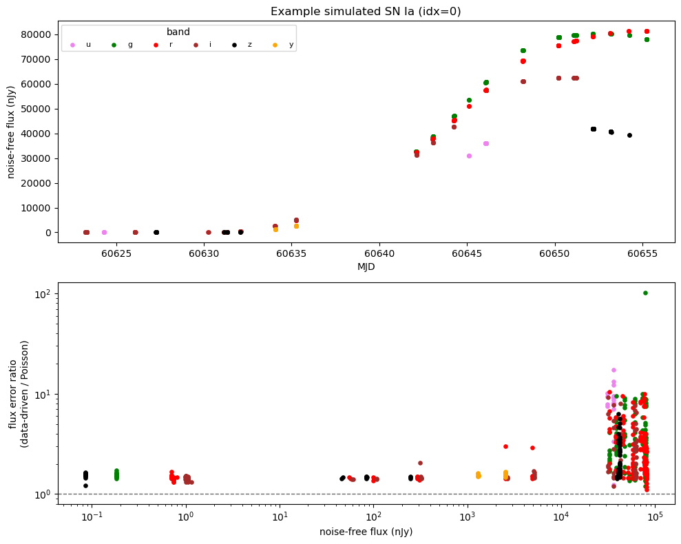
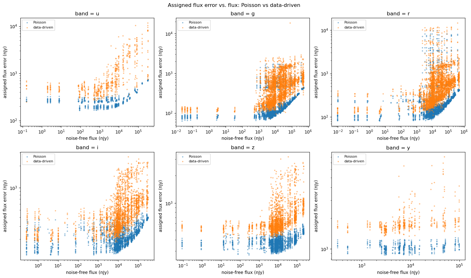
Now we compare the flux errors the two models assign across all simulated observations in each band. Any offset between the two point clouds shows where the data-driven model differs from the Poisson prediction.

def stack_obs(lc):
    """Stack all observations from a simulated-lightcurve frame into flat arrays."""
    filt, flux, err = [], [], []
    for i in range(len(lc)):
        row = lc.iloc[i]["lightcurve"]
        filt.append(np.asarray(row["filter"], dtype=str))
        flux.append(np.asarray(row["flux_perfect"], dtype=float))
        err.append(np.asarray(row["fluxerr"], dtype=float))
    return np.concatenate(filt), np.concatenate(flux), np.concatenate(err)


f_p, flux_p, err_p = stack_obs(lc_poisson)
f_z, flux_z, err_z = stack_obs(lc_pzflow)

fig, axes = plt.subplots(2, 3, figsize=(15, 9))
for ax, band in zip(axes.ravel(), BANDS):
    mp = f_p == band
    mz = f_z == band
    if not mp.any():
        ax.set_title(f"{band} (no obs)")
        continue
    ax.scatter(flux_p[mp], err_p[mp], s=4, alpha=0.4, label="Poisson")
    ax.scatter(flux_z[mz], err_z[mz], s=4, alpha=0.4, label="data-driven")
    ax.set_xscale("log")
    ax.set_yscale("log")
    ax.set_title(f"band = {band}")
    ax.set_xlabel("noise-free flux (nJy)")
    ax.set_ylabel("assigned flux error (nJy)")
    ax.legend(fontsize=8)
fig.suptitle("Assigned flux error vs. flux: Poisson vs data-driven")
fig.tight_layout()
plt.show()

Conclusion

We collected a flux-stratified training set from real Rubin DP1 forced photometry with LSDB, trained a pzflow model to generate flux errors from the flux and observing metadata, and used it as a drop-in noise model in a LightCurveLynx SN Ia simulation. The resulting PZFlowNoiseModel can be used like any other noise model, so the same approach extends to other source models and surveys.

A few things to revisit when adapting this notebook to your own science case:

• Which photometry to model: difference-image (psfDiffFlux, used here) or science-image (psfFlux), and at which positions (see the discussion in Part 1).

• The psfDiffFlux >= 0 filtering (Part 1.4) and the flux floor applied at simulation time (Part 3.3).

• The flux-stratification scheme and the TARGET_ROWS budget (Part 1.5).

• The pzflow training hyperparameters, passed through learn_pzflow_noise_model.