Simulations

Introduction

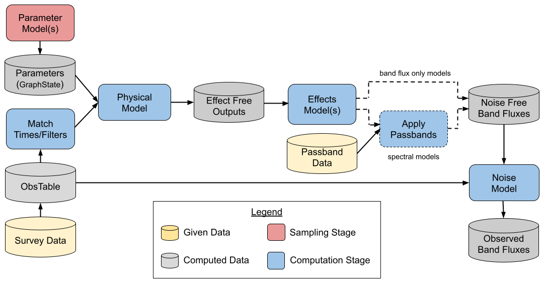
LightCurveLynx simulation components

The LightCurveLynx simulation function is designed to produce multiple samples from single population of objects and their observed light curves as determined by given survey information. The main step includes the following components:

• A statistical simulation step where parameters (and hyperparameters) of the modeled phenomenon are drawn from one or more prior distributions.

• A mathematical model that defines the properties of the time-domain light source, which can also include a host-galaxy model, and is used to generate the noise-free light curves (given the sampled parameters).

• SurveyInfo contains the survey information such as survey strategy, observing conditions, instrument characteristics, filter characteristics, and noise model. It is a wrapper around other specific data structures such as ObsTable and PassbandGroup.

• A set of predefined effects, such as dust extinction and detector noise, are applied to the noise-free light curves to produce realistic light curves.

To perform a simulation that includes different populations of objects, the user would run the core simulate function multiple times–once for each population. The results can then be concatenated together to provide a full set of observations.

For an overview of the package, we recommend starting with the notebooks in the “Getting Started” section of the notebooks page. The glossary provides definitions of key terms, such as GraphState, Node, Parameter, ParameterizedNode, BasePhysicalModel, BandfluxModel, and SEDModel.

Getting Started with a New Simulation

When starting a new simulation there are a few key questions to ask (in this order):

1. What do you want to simulate (supernova, kilanova, AGN, etc.)? The answer to this question determines the class you use to create the model object. For example, if you want to simulate a kilanova using the redback package, you would start by creating RedbackWrapperModel object.

2. What parameters does your model have? And how do you want to set them? The answers to these questions determine how you set the parameters of the model object. All parameters within a model are set using arguments in the object’s constructors.

3. What effects do you want to apply to the light coming from this object? The answer to this question will determine which effect objects you create and add to the object.

4. Under what conditions do you want to observe this object? What is your viewing cadence and instrument noise characteristics? In short, which survey are you using?

Defining a parameterized model

The core idea behind LightCurveLynx is that we want to generate light curves from parameterized models of astronomical objects/phenomena. Users do this by creating model objects that are subclasses of the BasePhysicalModel` class. This object provides the recipe for computing the noise-free light curves given values for its parameters. By providing a distribution of parameter values into the model, users can simulate an entire population of these objects. For example, they could use the SALT2JaxModel with parameterized values of c, x0, and x1 to simulate a population of Type Ia supernovae.

my_model = SALT2JaxModel(c=..., x0=..., x1=...)

In addition to the built-in models, the software provides wrappers to common modeling packages such as:

• BAGLE - a package for gravitational microlensing events modelling (example).

• bayesn - A package for hierarchical modeling of a Type Ia supernova (example).

• PyLIMA - A package for flexible micro-lensing event simulations (example).

• redback - A package for simulating and fitting a range of cosmological phenomena (example).

• sncosmo - A package for simulating supernovae.

• synphot - A package for simulating photometric observations (example).

• VBMicrolensing - A package for gravitational microlensing events using the advanced contour integration method (example).

LightCurveLynx also allows users to load and sample pre-generated light curves, such as the LCLIB (example) and SIMSED (example) formats used by SNANA. This allows users to simulate from populations of light curves that either come from real observations or from other modeling packages (such as SNANA).

Finally users can create their own models. See the custom models page or the adding new model types notebook for more details.

Parameterization

Users set the model’s parameters using the arguments of the model’s constructor. Parameters can be set to be static (a constant) or computed from a given distribution or function (which itself can have parameters). This flexibility allows the model’s parameters to be defined by a hierarchical model that can be visualized by a Directed Acyclic Graph (DAG). This means that the parameters to our physical model, such as a type Ia supernova, can themselves be sampled based on distributions of hyperparameters. For example, a simplified SNIa model with a host component can have the following DAG:

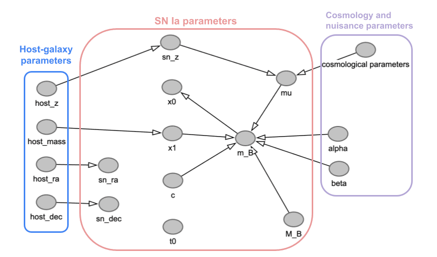
An example DAG for a SNIa model

In this example, the parameter c is drawn from a predefined distribution, while the parameter x1 is drawn from a distribution that is itself parameterized by the host_mass parameter.

Each sample during simulation corresponds to a new simulated object – all parameters are resampled and used to compute the flux density for that object. LightCurveLynx handles the sequential processing of the graph so that all parameters are consistently sampled for each object.

At the heart of the sampling system is the concept of a ParameterizedNode which is a node that takes settable parameters and produces values for other parameters. Many objects in LightCurveLynx are such nodes, including the BasePhysicalModel`. While this framework provides a powerful and extensible system for generating the DAGs, most users will not need to know the details. Instead LightCurveLynx provides a large set of predefined nodes that perform common operations. A few examples include:

• Sampling from a statistical distribution (e.g., NumpyRandomFunc and ScipyRandomDist)

• Sampling (RA, dec) from the footprint of a survey (e.g., ObsTableUniformRADECSampler and ApproximateMOCSampler)

• Performing basic math operations (e.g., BasicMathNode)

• Sampling from a given set of values (e.g., GivenValueList and TableSampler)

The directory /math_nodes contains many additional functions.

All most users will need to know is that the arguments passed to a model’s constructor can take values as:

• constants

• the output of a node that computes some value (e.g., NumpyRandomFunc)

• or the attribute of a another node.

See the Introduction notebook and sampling notebook for details on how to define the parameter DAG. The nodebook sampling positions provides a deeper dive into nodes that sample positions from a survey footprint.

Generating light curves

Sample light curves for a population are generated with a multiple step process. First, the object’s parameter DAG is sampled to get concrete values for each parameter in the model. This combination of parameters is called the graph state (and is stored in a GraphState object), because it represents the sampled state of the DAG.

Next, the ObsTable is used to determine at what times and in which bands the object will be evaluated. These times and wavelengths are based into the object’s evaluate_sed() function (for spectral level models) or evaluate_bandfluxes() (for band flux level models) along with the graph state. These functions handle the mechanics of the simulation, such as applying redshifts to both the times and wavelengths and handling any requested extrapolations outside the model’s valid time or wavelength range.

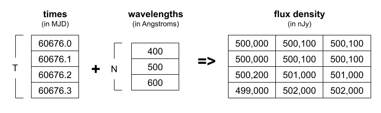
An example of the compute_sed function

Additional effects can be applied to the noise-free light curves to produce more realistic light curves. The effects are applied in two batches. Rest frame effects are applied to the flux densities in the rest frame. The flux densities are then converted to the observer frame where the observer frame effects are applied.

Finally, if the the raw flux densities are at the spectral level, they are integrated over the bandpasses to obtain the bandflux level values using the PassbandGroup.

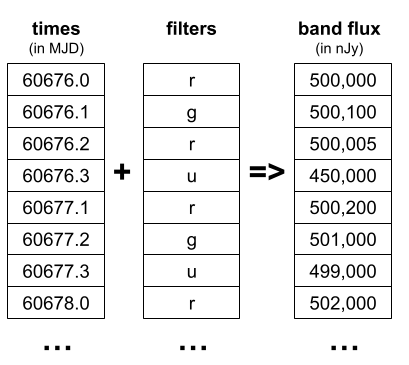
Generating band flux curves

All models provide a helper function, evaluate_bandfluxes(), that wraps the combination of evaluation and integration with the passbands. This function takes the passband information, a list of times, and a list of filter names. It returns the band flux at each of those times in each of the filters.

An example of the evaluate_bandfluxes function

In addition to being a convenient helper function for spectral models, generating the data at the band flux level allows certain models to skip spectral-level flux density generation. In particular a BandfluxModel is a subclass of the PhysicalModel whose computation is only defined at the band flux level. An example of this are models of empirically fit light curves, such as those from LCLIB. Since we do not have the underlying SEDs for these types of models, so we can only work with them at the band flux level. See the lightcurve template model for an example of this type of model.

Note that most models in LightCurveLynx operate at the spectral level and we strongly encourage new models to produce spectral-level information where possible. Working at the finer grained level allows more comprehensive and accurate simulations, such as accounting for wavelength and time compression due to redshift. The models that generate band fluxes directly will not account for all of these factors.

Running a Full Simulation

To run a full simulation, users call the simulate_lightcurves() function, which handles the parameter sampling, matching with ObsTable positions, the full density simulation (including effects), application of noise, etc. The function takes the model object to simulation, the number of samples to generate, and the survey information (SurveyInfo). It returns a nested pandas DataFrame as described in the Results and Output documentation page, which includes both the sampled parameters and the resulting light curves for each simulated object.

results = simulate_lightcurves(model, num_samples, survey_info)

The simulate_lightcurves() function has many additional arguments to allow the user to control various aspects of the simulation. These include:

• obs_time_window_offset and rest_time_window_offset which limit simulation to windows around the (observer and rest-frame respectively) t0 of the model.

• obstable_save_cols, param_cols, and save_full_filter_names which allow users to save additional context information about the simulation in the results.

• output_file_path which allows users to save the results to a file instead of returning them directly.

• executor, batch_size, and num_jobs which allow users to run the simulation in parallel. See the section on parallelization below for more details.

• rng which allows users to control the randomness of the simulation by passing in a predefined random number generator. See the section on controlling randomness below for more details.

Examples

After loading the necessary information (such as PassbandGroup and ObsTable), and defining the physical model for what we are simulating, we can generate light curves with realistic cadence and noise.

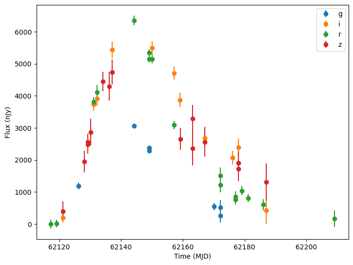
Simulated light curves of SNIa from LSST

See our selection of tutorial notebooks for further examples.

Controlling Randomness

LightCurveLynx allows the user to control randomness by passing in a predefined random number generator to simulate_lightcurves() via the rng parameter. If the user provides a random number generator with a fixed seed, then the parameters sampled throughout the simulation are effectively predefined and identical between simulations.

my_rng = np.random.default_rng(42)

If the provided random number generator does not use a fixed seed (or no rng argument is provided), the parameters will vary from run to run.

Simulating from Multiple Surveys

LightCurveLynx can simulate observations from multiple surveys in a single run by passing a list of SurveyInfo objects to the simulate_lightcurves() function. The parameter space is sampled once for each simulated object, so the observations in each survey are consistent with respect to the parameterization. The times of observation and filters used are determined by each survey. And the bandflux is computed using that survey’s passbands.

For an example see the Simulating from Multiple Surveys notebook.

Running in Parallel

Simulations can be performed in parallel by providing a concurrent.futures.Executor object. This object can be a built-in parallelization method, such as ThreadPoolExecutor or ProcessPoolExecutor, or other libraries, such as dask or ray. Note that each process will load a full version of all the data, so they may be memory intensive.

NOTE: Not all subpackages work with distributed computation yet. If you get an error about not being able to pickle an object, please let the LightCurveLynx team know so we can investigate.

The parallelization notebook provides an example of how to use LightCurveLynx to run simulations in parallel including using dask and ray.

Results and Output

The results of a simulation are returned as a nested-pandas DataFrame. For details on the structure of the output and how to save it, see the Results and Output documentation page.