Reading SNANA SED Models

In this notebook we look at how we can read in SED templates generated by SNANA and simulate them under different observing cadences and noise conditions.

from astropy.cosmology import Planck18
import numpy as np

from lightcurvelynx import _LIGHTCURVELYNX_BASE_DATA_DIR
from lightcurvelynx.astro_utils.passbands import PassbandGroup
from lightcurvelynx.math_nodes.np_random import NumpyRandomFunc
from lightcurvelynx.math_nodes.ra_dec_sampler import ApproximateMOCSampler
from lightcurvelynx.models.sed_template_model import SIMSEDModel
from lightcurvelynx.obstable.opsim import OpSim
from lightcurvelynx.simulate import simulate_lightcurves
from lightcurvelynx.survey_info import SurveyInfo
from lightcurvelynx.utils.plotting import plot_lightcurves

Load Data Files

We start by loading the files we will need for running the simulation: the ObsTable of survey information and the passband information. Both of these live in the data/ directory in the root directory. Note that nothing in this directory is saved to github, so the files will need to be manaully downloaded initially.

For Rubin, a large number of OpSims can be found at https://s3df.slac.stanford.edu/data/rubin/sim-data/. You can download an OpSim manually or using the from_url() helper function:

opsim_url = “https://s3df.slac.stanford.edu/data/rubin/sim-data/sims_featureScheduler_runs5.3/baseline/baseline_v5.3.0_10yrs.d”

opsim_data = OpSim.from_url(opsim_url)

In this example we use an artificial opsim that looks at the same region of sky every night for 3 months (Jan 1, 2027 through April 1, 2027). Using a rotation of the “g”, “r”, “i”, and “z” filters.

filters_options = ["g", "r", "i", "z"]

times = np.arange(61406, 61496, 1)
values = {
    "observationStartMJD": np.array(times),
    "fieldRA": np.full(len(times), 30.0),  # Fixed RA for all viewings
    "fieldDec": np.full(len(times), -30.0),  # Fixed dec for all viewings
    "zp_nJy": np.random.normal(loc=0.6, scale=0.1, size=len(times)),  # Random zeropoint around 0.6 nJy
    "seeingFwhmEff": np.random.normal(
        loc=1.2, scale=0.1, size=len(times)
    ),  # Random seeing FWHM around 1.2 arcsec
    "skyBrightness": np.random.normal(
        loc=21.0, scale=0.5, size=len(times)
    ),  # Random sky brightness around 21 mag/arcsec^2
    "nexposure": np.full(len(times), 2),  # 2 exposures per visit
    "exptime": np.full(len(times), 30.0),  # 30 second exposures
    "filter": np.array([filters_options[i % 4] for i in range(len(times))]),
}
opsim_db = OpSim(values)

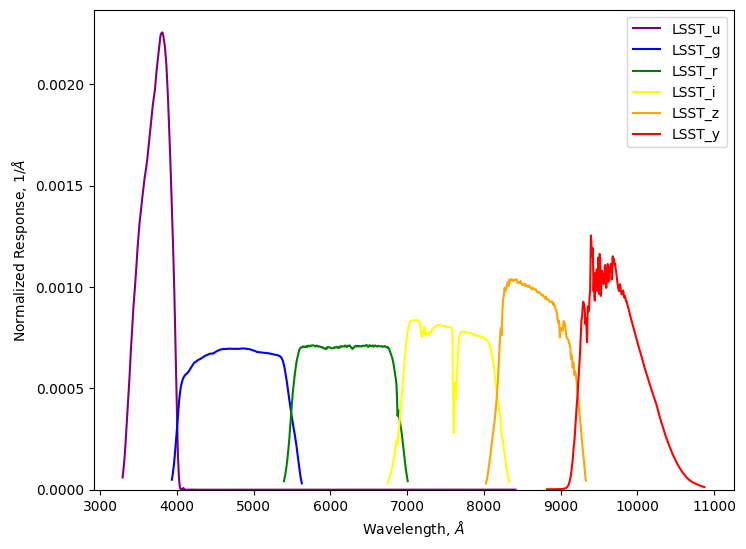
Load the passband information, using the same filters. For most models the passband information will be used to convert the SED into bandfluxes. However, since we already have light curves at the bandflux level, we will just generate observations directly from those.

# Load the passband data for the griz filters only.
table_dir = _LIGHTCURVELYNX_BASE_DATA_DIR / "passbands" / "LSST"
passband_group = PassbandGroup.from_preset(
    preset="LSST",
    units="nm",
    trim_quantile=0.001,
    delta_wave=1,
    table_dir=table_dir,
)
passband_group.plot()

Create the model

We want to create models based on SED-level data generated by SNANA. In this example we use the SIMSED.TDE-MOSFIT data set from https://zenodo.org/records/2612896 which contains 699 SED templates in SIMSED format. Note that this data is not stored in the github repository and must be downloaded separately from zenodo.

Each template consists of sampled SED values (in erg/cm²/s/Å as seen from 10 pc in rest-frame) for a grid of times and wavelengths. An additional SED.INFO provides global information for the templates, such as the flux scaling factor. LightCurveLynx handles all the internal conversions, so results are produced in the same units as other models (nJy).

The SIMSEDModel object loads each SED template in a target directory. It also reads the corresponding SED.INFO file to extract relevant data set wide parameters, such as the flux scaling factor. New observations are created by randomly choosing one of the SED templates and interpolating it the query times and wavelengths. The starting time of the activity is controlled by the t0 parameter in the model. So we can generate a simulation where the object’s activity starts halfway through our observations.

Since SIMSEDModel is a PhysicalModel, we can specify other parameters such as the RA and dec. In this examples, we generate this position information by sampling from the OpSim fields (using an ApproximateMOCSampler node). We sample the starting time of the event within the first 20 days of the survey coverage. Luminosity distance is computed automatically from the combination of redshift (which is random from [0.1, 0.6]) and the Planck18 cosmology.

# We create the sampling area using a MOC that covers the region observed in the OpSim.
coverage_moc = opsim_db.build_moc(radius=1.0)  # 1 degree radius around each field center
ra_dec_sampler = ApproximateMOCSampler(coverage_moc)

# Use a uniform sampler for the starting time (t0) of activity. All events will
# start within the first 20 days of the survey (between MJD 61406 and 61426).
time_sampler = NumpyRandomFunc("uniform", low=61406, high=61426, node_label="time_sampler")

source = SIMSEDModel.from_dir(
    # The directory containing the SIMSED files.
    _LIGHTCURVELYNX_BASE_DATA_DIR / "model_files" / "SIMSED.SNIbc-MOSFIT",
    # The other parameters for the model.
    ra=ra_dec_sampler.ra,
    dec=ra_dec_sampler.dec,
    t0=time_sampler,
    node_label="source",
    redshift=NumpyRandomFunc("uniform", low=0.1, high=0.6),
    cosmology=Planck18,
)

Loading: 100%|██████████| 699/699 [00:15<00:00, 45.34file/s]

Generate the simulations

We can now generate random simulations with all the information defined above. The simulate_lightcurves function takes three parameters: the source from which we want to sample (here the collection of SED templates), the number of results to simulate (1,000), and the passband information.

survey_info = SurveyInfo(obstable=opsim_db, passbands=passband_group, survey_name="LSST")

lightcurves = simulate_lightcurves(source, 1_000, survey_info)

Simulating: 100%|██████████| 1000/1000 [00:01<00:00, 501.00obj/s]

The results are written in the nested-pandas format for easy analysis. Each row corresponds to a single simulated object, with a unique id, ra, dec, etc. The column params include all internal state, including hyperparameter settings, that was used to generate this object. The nested lightcurve column contains the times, filters, and fluxes for each observation of that object.

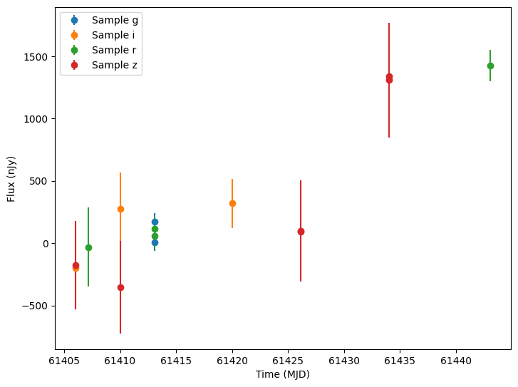
We can extract the light curve for a single simulated object and plot it.

lightcurve0 = lightcurves.iloc[0]["lightcurve"]
plot_lightcurves(
    fluxes=np.asarray(lightcurve0["flux"], dtype=float),
    times=np.asarray(lightcurve0["mjd"], dtype=float),
    fluxerrs=np.asarray(lightcurve0["fluxerr"], dtype=float),
    filters=np.asarray(lightcurve0["filter"], dtype=str),
)

<Axes: xlabel='Time (MJD)', ylabel='Flux (nJy)'>

More Realistic OpSim

Let’s repeat the simulation using a real Rubin OpSim to get more realistic cadence and noise. We filter the time range to the same three month coverage as the above. We also remove the filters that we will not use.

# Load the OpSim data.
opsim_db = OpSim.from_db(_LIGHTCURVELYNX_BASE_DATA_DIR / "opsim" / "baseline_v5.3.0_10yrs.db")
print(f"Loaded OpSim with {len(opsim_db)} rows.")

time_mask = (opsim_db["observationStartMJD"] >= 61406) & (opsim_db["observationStartMJD"] < 61496)
filter_mask = np.isin(opsim_db["filter"], filters_options)
opsim_db = opsim_db.filter_rows(time_mask & filter_mask)
print(f"Filtered OpSim has {len(opsim_db)} rows.")

survey_info = SurveyInfo(obstable=opsim_db, passbands=passband_group)

Loaded OpSim with 2146797 rows.
Filtered OpSim has 52641 rows.

Instead of randomly sampling RA, dec, and time, we will use values from the OpSim to ensure that we observe the point of interest. We give the start time of the event as 10 days after the start of the survey.

source = SIMSEDModel.from_dir(
    # The directory containing the SIMSED files.
    _LIGHTCURVELYNX_BASE_DATA_DIR / "model_files" / "SIMSED.SNIbc-MOSFIT",
    # The other parameters for the model.
    ra=opsim_db["ra"].iloc[0],
    dec=opsim_db["dec"].iloc[0],
    t0=61416,
    node_label="source",
    redshift=NumpyRandomFunc("uniform", low=0.1, high=0.6),
    cosmology=Planck18,
)

Loading: 100%|██████████| 699/699 [00:15<00:00, 46.53file/s]

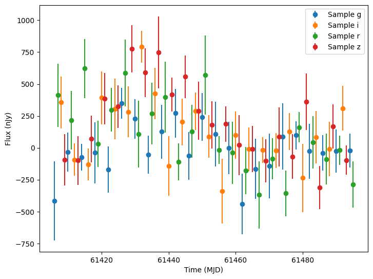
We run one additional simulation for the new point.

lightcurves = simulate_lightcurves(source, 1, survey_info)
lightcurve0 = lightcurves.iloc[0]["lightcurve"]
plot_lightcurves(
    fluxes=np.asarray(lightcurve0["flux"], dtype=float),
    times=np.asarray(lightcurve0["mjd"], dtype=float),
    fluxerrs=np.asarray(lightcurve0["fluxerr"], dtype=float),
    filters=np.asarray(lightcurve0["filter"], dtype=str),
)

Simulating: 100%|██████████| 1/1 [00:00<00:00, 303.14obj/s]

<Axes: xlabel='Time (MJD)', ylabel='Flux (nJy)'>