AGN Damped Random Walk Example
In this notebook we run a simulation of a damped random walk AGN variability model built-in with LightCurveLynx. The model is similiar to one used in ELAsTiCC simulations, it uses the standard disk spectrum as the SED “baseline” and perturbs it stochastically.
[1]:
import numpy as np

from astropy.cosmology import Planck18
from lightcurvelynx.base_models import FunctionNode
from lightcurvelynx.math_nodes.np_random import NumpyRandomFunc
from lightcurvelynx.math_nodes.ra_dec_sampler import ObsTableRADECSampler
from lightcurvelynx.math_nodes.scipy_random import SamplePDF
from lightcurvelynx.models.agn import AGN
from lightcurvelynx.obstable.opsim import OpSim
from lightcurvelynx.simulate import simulate_lightcurves
from lightcurvelynx.survey_info import SurveyInfo
from lightcurvelynx.utils.plotting import plot_lightcurves
Create Parameter Distributions
With LightCurveLynx model parameters may be both fixed numerical values or to be drawn from random distributions. Here we create few of AGN model parameters.
[3]:
# Draw redshift from the uniform distribution
redshift = NumpyRandomFunc("uniform", low=0.1, high=1.0)

# Draw decimal logarithm of the black hole mass (in solar masses)
# from the uniform distribution
lg_bh_mass = NumpyRandomFunc("uniform", low=7.0, high=9.0)
# Transform to mass in solar masses
bh_mass = FunctionNode(
    lambda lg_mass: 10**lg_mass,
    lg_mass=lg_bh_mass,
    node_label="bh_mass",
)


# Eddington ratio for the accretion rate, e.g. accretion rate to critical value ratio
# First, we define a PDF function, for "blue" galaxies, see
# https://github.com/burke86/imbh_forecast/blob/master/var.ipynb
# https://ui.adsabs.harvard.edu/abs/2019ApJ...883..139S/abstract
# https://iopscience.iop.org/article/10.3847/1538-4357/aa803b/pdf
def edd_ratio_pdf(value):
    xi = 10**-1.65
    lambda_br = 10**-1.84
    delta1 = 0.471 - 0.7
    delta2 = 2.53
    min_lambda = 0.01
    max_lambda = 1.0
    value = np.asarray(value)
    fill_mask = (value >= min_lambda) & (value <= max_lambda)
    prob = np.zeros_like(value)
    prob[fill_mask] = xi / (
        (value[fill_mask] / lambda_br) ** delta1 + (value[fill_mask] / lambda_br) ** delta2
    )
    return prob


# We use a special random node to sample from this PDF
edd_ratio = SamplePDF(edd_ratio_pdf)

# We use a special distribution to draw positions from the survey coverage area
radec = ObsTableRADECSampler(
    obstable,
    radius=3.0,  # degrees
    node_label="ra_dec_sampler",
)
Create a Model and Run Simulations
It is time to create the model and simulate few light curves!
[4]:
model = AGN(
    # Reference time is not important for a stochastic model
    t0=obstable.time_bounds()[0],  # reference date, the survey start
    blackhole_mass=bh_mass,  # black hole mass in solar masses
    edd_ratio=edd_ratio,  # accretion rate to critical accretion rate raio
    redshift=redshift,
    ra=radec.ra,
    dec=radec.dec,
    cosmology=Planck18,
)

# Make it reproducible
rng = np.random.default_rng(42)

df = simulate_lightcurves(
    model=model,
    num_samples=10,
    survey_info=survey_info,
    param_cols=[
        "bh_mass.lg_mass",
        "AGN_0.edd_ratio",
    ],
    rng=rng,
)
# params is too large to show =)
df.drop(columns=["params"])
Simulating: 100%|██████████| 10/10 [00:00<00:00, 10.49obj/s]
[4]:
| id | ra | dec | nobs | t0 | z | bh_mass_lg_mass | AGN_0_edd_ratio | lightcurve | ||||||||||||||||
|---|---|---|---|---|---|---|---|---|---|---|---|---|---|---|---|---|---|---|---|---|---|---|---|---|
| 0 | 0 | 139.858196 | 5.627499 | 668 | 61208.201382 | 0.275175 | 7.378943 | 0.040020 |
|
|||||||||||||||
| 1 | 1 | 20.117732 | -12.482954 | 712 | 61208.201382 | 0.520049 | 7.259843 | 0.017156 |
|
|||||||||||||||
| 2 | 2 | 49.830898 | -27.321914 | 706 | 61208.201382 | 0.139423 | 7.951410 | 0.014922 |
|
|||||||||||||||
| 3 | 3 | 81.318890 | -15.613943 | 711 | 61208.201382 | 0.238861 | 7.453819 | 0.028611 |
|
|||||||||||||||
| 4 | 4 | 23.753189 | -10.960924 | 630 | 61208.201382 | 0.714744 | 8.339628 | 0.012180 |
|
|||||||||||||||
| 5 | 5 | 280.082832 | -41.721618 | 925 | 61208.201382 | 0.770286 | 7.874304 | 0.013223 |
|
|||||||||||||||
| 6 | 6 | 197.537710 | -33.589037 | 767 | 61208.201382 | 0.970759 | 8.665356 | 0.010108 |
|
|||||||||||||||
| 7 | 7 | 295.161710 | -67.694582 | 697 | 61208.201382 | 0.393243 | 8.400530 | 0.037724 |
|
|||||||||||||||
| 8 | 8 | 11.187587 | -73.916434 | 657 | 61208.201382 | 0.433414 | 7.624733 | 0.027525 |
|
|||||||||||||||
| 9 | 9 | 162.854353 | -1.282532 | 733 | 61208.201382 | 0.522600 | 8.664520 | 0.030152 |
|
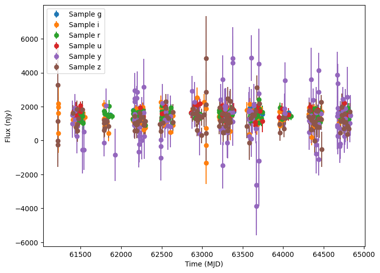
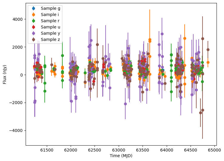
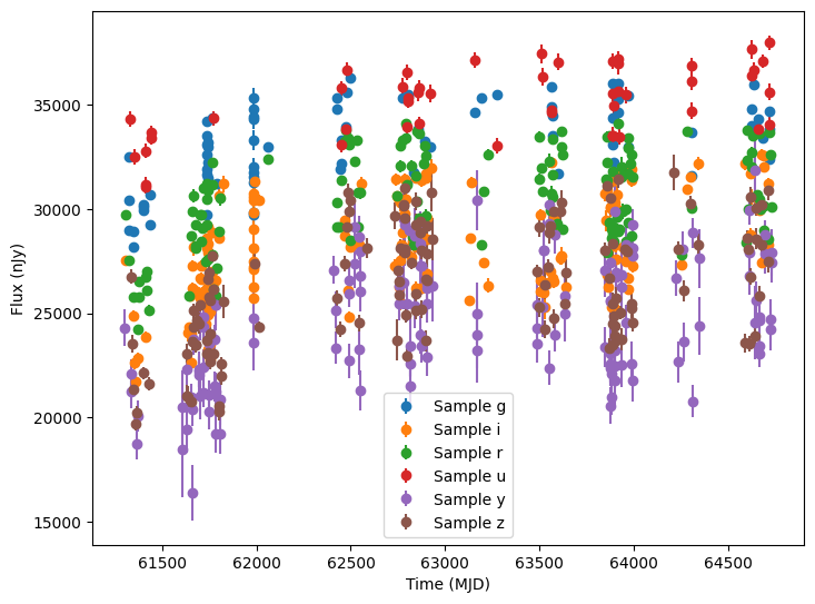
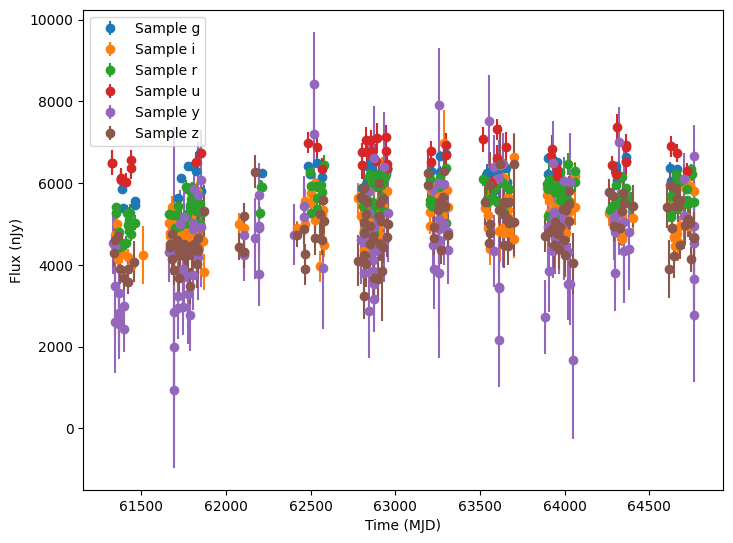
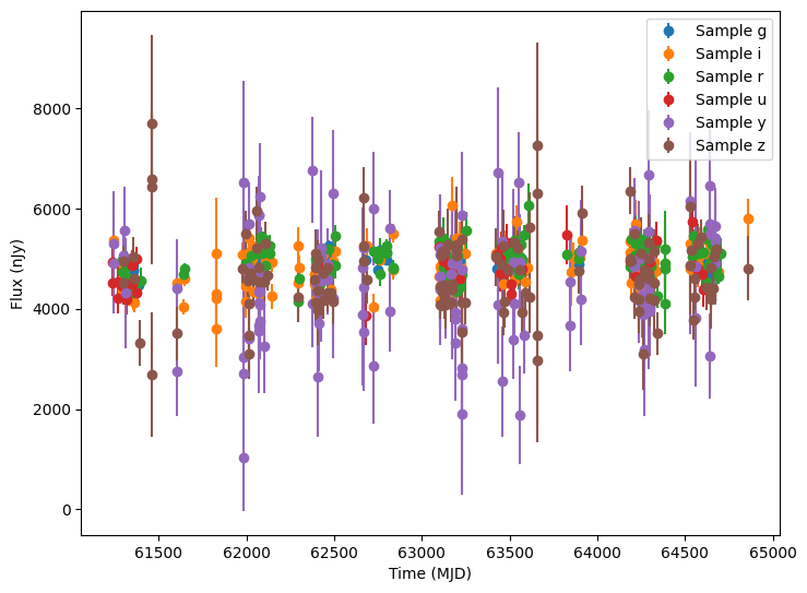
Plot few light curves
[5]:
for idx in range(5):
    # Extract the row for this object.
    row = df.iloc[idx]
    lc = row["lightcurve"]

    plot_lightcurves(
        fluxes=lc["flux"],
        times=lc["mjd"],
        fluxerrs=lc["fluxerr"],
        filters=lc["filter"],
    )