Simulating SNIa with Rubin Opsim

In this notebook, we demonstrate how to simulate a Type Ia supernova using toy parameter distributions and the Rubin OpSim cadence.

import numpy as np
from lightcurvelynx import _LIGHTCURVELYNX_BASE_DATA_DIR
from lightcurvelynx.astro_utils.snia_utils import (
    DistModFromRedshift,
    HostmassX1Func,
    X0FromDistMod,
)
from lightcurvelynx.math_nodes.np_random import NumpyRandomFunc
from lightcurvelynx.math_nodes.ra_dec_sampler import ApproximateMOCSampler
from lightcurvelynx.models.sncosmo_models import SncosmoWrapperModel
from lightcurvelynx.models.snia_host import SNIaHost
from lightcurvelynx.obstable.opsim import OpSim
from lightcurvelynx.simulate import simulate_lightcurves
from lightcurvelynx.survey_info import SurveyInfo
from lightcurvelynx.utils.plotting import plot_lightcurves

Load Data Files

We start by loading the files we will need for running the simulation, the OpSim database. This file is not included in the github repository, so the user must manually download the file. In this example, we use the baseline_v5.3.0_10yrs.db data file, which we have pre-downloaded to a local directory data/opsim.

For Rubin, a large number of OpSims can be found at https://s3df.slac.stanford.edu/data/rubin/sim-data/. You can download an OpSim manually or using the from_url() helper function:

opsim_url = “https://s3df.slac.stanford.edu/data/rubin/sim-data/sims_featureScheduler_runs3.4/baseline/baseline_v3.4_10yrs.db” opsim_data = OpSim.from_url(opsim_url)

Since we are using a standard survey type (LSST), we can just pass the name to the SurveyInfo info constructor and have it load the default passbands and noise model.

# Load the OpSim data. You will need to have downloaded the OpSim data to a local directory and set the
# path accordingly.
opsim_db = OpSim.from_db(_LIGHTCURVELYNX_BASE_DATA_DIR / "opsim" / "baseline_v5.3.0_10yrs.db")

t_min, t_max = opsim_db.time_bounds()
print(f"Loaded OpSim with {len(opsim_db)} rows and times [{t_min}, {t_max}]")

survey_info = SurveyInfo(obstable=opsim_db, survey_name="LSST")

Loaded OpSim with 1844571 rows and times [61208.201382236985, 64860.44487408427]

Create the model

To generate simulationed lightcurves we need to define the proporties of the object from which to sample, including RA, Dec, and the logmass. We recommend pzflow models as a good way of modeling this distribution. As shown in the pzflow example notebook, users can train, load, and query pzflow models.

To keep this notebook simple and reproducible, we use a simpler sampling strategy. We sample (RA, Dec, t0) uniformly from the footprint of the survey, redshift sampled uniformly [0.1, 0.6] and the logmass as a normal distribution centered on 9.

# Create a MOC sampler for the survey. This will be used to sample positions on the sky that are consistent
# with the survey's footprint.
pos_sampler = ApproximateMOCSampler.from_obstable(opsim_db, depth=8)

# Sample the t0 parameter uniformly from the survey's time bounds.
t0_sampler = NumpyRandomFunc("uniform", low=t_min, high=t_max)

# Sample the redshift uniformly between 0.1 and 0.6. This is just an example, and can be changed to match the expected
# redshift distribution of the SNe Ia in the survey.
redshift_sampler = NumpyRandomFunc("uniform", low=0.1, high=0.6)

# Sample the logmass as normal distribution with mean 9 and std 1. This is just an example, and can be changed
# to match the expected distribution of host masses.
logmass_sampler = NumpyRandomFunc("normal", loc=9, scale=1)

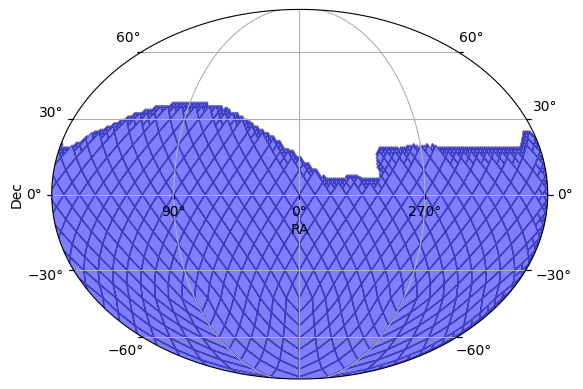
We can see the footprint from which we will sample using the plot_footprint function.

pos_sampler.plot_footprint()

(<Figure size 640x480 with 1 Axes>, <WCSAxes: >)

Given these samplers, we can create a model of the host galaxy.

# Create a model for the host of the SNIa. The attributes will be sampled via
# the different sampler nodes. So each host instantiation will have its own properties.
host = SNIaHost(
    ra=pos_sampler.ra,  # The RA portion of the position sample.
    dec=pos_sampler.dec,  # The Dec portion of the position sample.
    hostmass=logmass_sampler,  # The ouput of the logmass sampler.
    redshift=redshift_sampler,  # The output of the redshift sampler.
    node_label="host",
)

Next we create the SNIa model itself. We use sncosmo’s SALT2 model with parameters randomly generated from toy distributions. Note that the function nodes, such as DistModFromRedshift, will compute value per row, so that the sampled distmod is consistent with that row’s redshift. This is an example of sampler chaining. For more detail see the advanced sampling notebook.

Some attributes are sampled relative to the host’s properties. In this case both RA and Dec are sampled using a normal distribution centered on the galaxy’s position. This is another example of chaining that makes the source’s position a noisy offset of the galaxy’s center.

# Create a function that will compute the distmod from the sampled redshift and given H0/Omega_m.
distmod_func = DistModFromRedshift(host.redshift, H0=73.0, Omega_m=0.3)

# Create a function that will compute the x1 parameter from the host mass.
x1_func = HostmassX1Func(host.hostmass)

# Sample c from a normal distribution with mean 0 and std 0.02.
c_func = NumpyRandomFunc("normal", loc=0, scale=0.02)

# Sample m_abs from a normal distribution with mean -19.3 and std 0.1.
m_abs_func = NumpyRandomFunc("normal", loc=-19.3, scale=0.1)

# Create a function that will compute the x0 parameter from the sampled distmod, x1, c, and m_abs.
x0_func = X0FromDistMod(
    distmod=distmod_func,
    x1=x1_func,
    c=c_func,
    alpha=0.14,
    beta=3.1,
    m_abs=m_abs_func,
)

source = SncosmoWrapperModel(
    "salt2-h17",  # Name of the sncosmo model to use.
    t0=NumpyRandomFunc("uniform", low=t_min, high=t_max),
    x0=x0_func,
    x1=x1_func,
    c=c_func,
    ra=NumpyRandomFunc("normal", loc=host.ra, scale=0.01),
    dec=NumpyRandomFunc("normal", loc=host.dec, scale=0.01),
    redshift=host.redshift,
    node_label="source",
)

Generate the simulations

We can now generate random simulations with all the information defined above:

• The source model we want to simulate (source)

• The number of samples to draw (1,000)

• The survey information (opsim, passband info, etc.)

The light curves are written in the nested-pandas format for easy analysis. For readability, we drop the “params” column which contains a dictionary representation of all the parameters used to create that sample.

lightcurves = simulate_lightcurves(source, 1_000, survey_info)
lightcurves = lightcurves.drop(columns=["params"])
lightcurves.head()

Simulating:   0%|          | 0/1000 [00:00<?, ?obj/s]/Users/jkubica/h/lightcurvelynx/src/lightcurvelynx/models/physical_model.py:535: UserWarning: Some times are less than the model's defined bounds and no time extrapolation is set. If this is not the intended, you can enable time extrapolation using the 'time_extrapolation' parameter.
  warnings.warn(
/Users/jkubica/h/lightcurvelynx/src/lightcurvelynx/models/physical_model.py:562: UserWarning: Some times are greater than the model's defined bounds and no time extrapolation is set. If this is not the intended, you can enable time extrapolation using the 'time_extrapolation' parameter.
  warnings.warn(
Simulating: 100%|██████████| 1000/1000 [00:02<00:00, 402.03obj/s]

	id	ra	dec	nobs	t0	z	lightcurve
0	0	255.398215	-16.631099	671	61514.671234	0.414334	mjd filter ... obs_idx is_saturated 61213.202154 y ... 2438 False +670 rows ... ... ... ...
1	1	320.217142	-28.327403	725	63130.281484	0.491512	mjd filter ... obs_idx is_saturated 61210.412281 u ... 1610 False +724 rows ... ... ... ...
2	2	158.157696	-22.971491	763	63111.123764	0.436109	mjd filter ... obs_idx is_saturated 61327.372269 i ... 47572 False +762 rows ... ... ... ...
3	3	178.049657	20.678286	13	62546.934400	0.554466	mjd filter ... obs_idx is_saturated 61470.254909 g ... 115306 False +12 rows ... ... ... ...
4	4	126.675337	-56.258802	222	63379.256980	0.521821	mjd filter ... obs_idx is_saturated 61366.293656 z ... 63554 False +221 rows ... ... ... ...

5 rows x 7 columns

Now let’s plot some random light curves

lightcurves = lightcurves.dropna(subset=["lightcurve"])
random_ids = np.random.choice(len(lightcurves), 3)

for random_id in random_ids:
    # Extract the row for this object.
    lc = lightcurves.iloc[random_id]

    # Unpack the nested columns (filters, mjd, flux, and flux error).
    lc_filters = np.asarray(lc["lightcurve"]["filter"], dtype=str)
    lc_mjd = np.asarray(lc["lightcurve"]["mjd"], dtype=float)
    lc_flux = np.asarray(lc["lightcurve"]["flux"], dtype=float)
    lc_fluxerr = np.asarray(lc["lightcurve"]["fluxerr"], dtype=float)

    ax = plot_lightcurves(
        fluxes=lc_flux,
        times=lc_mjd,
        fluxerrs=lc_fluxerr,
        filters=lc_filters,
    )

    # Get and plot a vertical line at the t0 value for this object.
    t0 = lightcurves.iloc[random_id]["t0"]
    ax.axvline(t0, color="k", linestyle="--", label="t0")
    ax.legend()

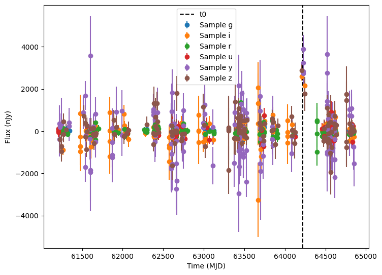
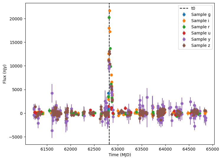
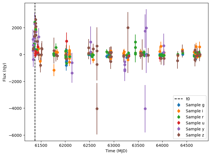
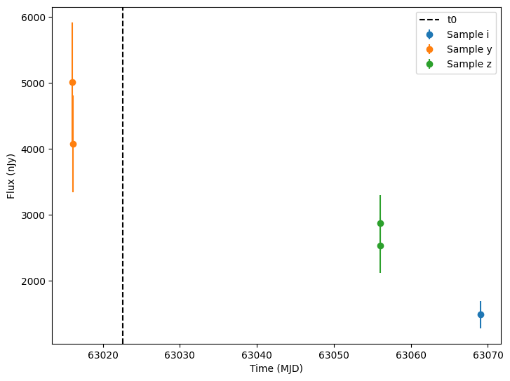
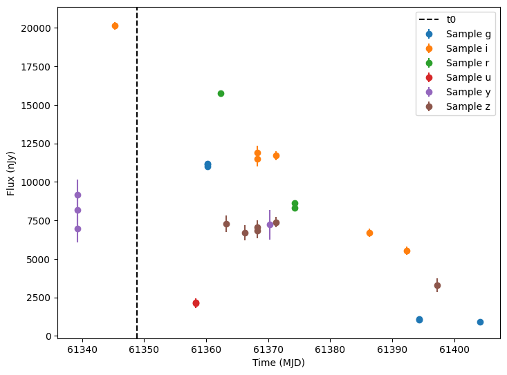
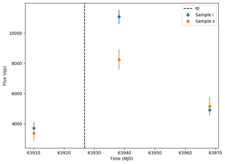
The plots above show the light curves of the supernova, but they comprise only a relative small amount of the total observational points. Most of the points are just the background noise (without the supernova light) and would generally not pass a detection threshold.

So let’s apply some detection thresholds and plot only detections. Specifically, we will use the flux and fluxerr columns to compute a signal to noise column. Then we filter anything with a signal to noise less than 5.

lightcurves["lightcurve.snr"] = lightcurves["lightcurve.flux"] / lightcurves["lightcurve.fluxerr"]
detections = lightcurves.query("lightcurve.snr > 5").dropna(subset=["lightcurve"])
random_ids = np.random.choice(len(detections), 3)

for random_id in random_ids:
    # Extract the row for this object.
    lc = detections.iloc[random_id]

    # Unpack the nested columns (filters, mjd, flux, and flux error).
    lc_filters = np.asarray(lc["lightcurve"]["filter"], dtype=str)
    lc_mjd = np.asarray(lc["lightcurve"]["mjd"], dtype=float)
    lc_flux = np.asarray(lc["lightcurve"]["flux"], dtype=float)
    lc_fluxerr = np.asarray(lc["lightcurve"]["fluxerr"], dtype=float)

    ax = plot_lightcurves(
        fluxes=lc_flux,
        times=lc_mjd,
        fluxerrs=lc_fluxerr,
        filters=lc_filters,
    )

    # Get and plot a vertical line at the t0 value for this object.
    t0 = detections.iloc[random_id]["t0"]
    ax.axvline(t0, color="k", linestyle="--", label="t0")
    ax.legend()