Wrapping Libraries - Bagle Example

This notebook is part of a series demonstrating how users can add support for their own simulation packages by adding simple wrappers. The example covered in this notebook is the Bagle Microlensing package. To run this notebook you will need to install Bagle. See the instructions here.

This notebook is based on the lightcurvelynx_BAGLE.ipynb notebook by Natasha Abrams and Katarzyna Kruszynska (2025).

Bagle

Bagle is a package for simulating and analyzing gravitational lensing effects, which includes functions to model the output of such event. For an introduction to bagle, see their tutorial notebook: https://github.com/MovingUniverseLab/BAGLE_Microlensing/blob/main/BAGLE_TUTORIAL.ipynb.

Bagle uses the bagle.model object to store the information and perform the computations for microlensing events. This is the object that we will want to wrap within a LightCurveLynx BasePhysicalModel so we can use it in the computation flow.

Let’s start by looking at how we can create and query a standard bagle model. The object’s constructor takes in the parameters as (order dependent) arguments. For example, we can create a PSPL_PhotAstrom_Par_Param1 (point source, point lens) object as:

from bagle import model

# Create the event model with given parameter.
event1 = model.PSPL_PhotAstrom_Par_Param1(
    1.0,  # mL (msun)
    61600,  # t0 (MJD)
    0.1,  # beta (mas)
    4000.0,  # dL (pc)
    4000.0 / 8000.0,  # dL/dS
    0.0,  # xS0_E (mas/yr)
    0.0,  # xS0_N (mas/yr)
    5.0,  # muL_E (mas/yr)
    10.0,  # muL_N (mas/yr)
    0.0,  # muS_E (mas/yr)
    0.0,  # muS_N (mas/yr)
    [1, 1, 1, 1, 1, 1],  # b_sff
    [23, 22, 21.5, 21, 20.5, 19.5],  # mag_src
    raL=270.66679,  # RA (deg)
    decL=-35.70483,  # Dec (deg)
)

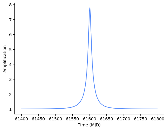
Given the model, we can query for outputs, such as the amplification level, over given times. Here we use 200.0 days before the given t0 to 200.0 days after it.

import matplotlib.pyplot as plt
import numpy as np

t = np.arange(61400.0, 61800.0, 1.0)

A = event1.get_amplification(t)
plt.plot(t, A)
plt.xlabel("Time (MJD)")
plt.ylabel("Amplification")

Text(0, 0.5, 'Amplification')

Most important for our case will be the model’s get_photometry() function which will return the magnitudes for a given filter at a given array of times. We can uses this as the basis for LightCurveLynx’s computation function with a few modifications. Most notably, LightCurveLynx uses fluxes in nJy, so we will need to convert the magnitudes.

Wrapping Bagle Models

To wrap a bagle model we need to design a subclass of LightCurveLynx’s BasePhysicalModel that:

1. constructs the bagle model,

2. sets its parameters, and

3. queries the flux that it produces (returning the results in nJy). Since bagle models operate on the bandflux level, we start by subclassing LightCuvreLynx’s BandfluxModel class.

We start using an alternative approach for creating a model object from the model name (given in Abrams and Kruszynska’s notebook) that loads the model from the library (using Python’s getattr() function) and assemble the parameters as a dictionary.

# Give the name of the class we will create.
model_name = "PSPL_PhotAstrom_Par_Param1"

# Define the parameters as a dictionary.
dL = 4000  # Distance to lens
dS = 8000  # Distance to source
parameter_dict = {
    "raL": 270.66679,
    "decL": -35.70483,
    "mL": 1,  # Msun (Primary lens current mass)
    "t0": 61600,  # mjd
    "beta": 0.1,
    "dL": dL,
    "dL_dS": dL / dS,
    "xS0_E": 0.0,  # arbitrary offset (arcsec)
    "xS0_N": 0.0,  # arbitrary offset (arcsec)
    "muL_E": 5.0,
    "muL_N": 10.0,
    "muS_E": 0.0,
    "muS_N": 0.0,
    "b_sff": [1, 1, 1, 1, 1, 1],
    "mag_src": [23, 22, 21.5, 21, 20.5, 19.5],
}

# Create the model object, by creating the model class by name and
# passing the parameters as a dictionary.
mod_class = getattr(model, model_name)
mod = mod_class(**parameter_dict)

To wrap this as a LightCurveLynx model, we will need two functions:

• __init__() - Set up the internal data and register the (settable) parameters.

• compute_bandflux() - Compute the flux values (in nJy) at given times and filters.

The model above specifies the b_sff and mag_src for the filters in the order: u, g, r, i, z, y. To make the mappings easier, we also define a class variable _filter_idx with dictionary mapping filter name to its index.

from lightcurvelynx.astro_utils.mag_flux import mag2flux
from lightcurvelynx.models.physical_model import BandfluxModel


class FixedBagleModel(BandfluxModel):
    """A wrapper for a Bagle model with a fixed set of parameters."""

    # Convenience mapping from filter name to index in the parameter list.
    _filter_idx = {"u": 0, "g": 1, "r": 2, "i": 3, "z": 4, "y": 5}

    def __init__(self, model_name, parameter_dict, **kwargs):
        # We start by extracting the parameter information needed for a general
        # physical model (base class).
        ra = parameter_dict["raL"]
        dec = parameter_dict["decL"]
        t0 = parameter_dict["t0"]

        # Call the parent class constructor to set up the model.
        super().__init__(ra=ra, dec=dec, t0=t0, **kwargs)

        # The create the bagle model object and set the parameters.
        self.model_name = model_name
        self.parameter_dict = parameter_dict
        mod_class = getattr(model, model_name)
        self.model_obj = mod_class(**parameter_dict)

    def compute_bandflux(self, times, filter, state):
        """Evaluate the model at the passband level for a single, given graph state and filter.

        Parameters
        ----------
        times : numpy.ndarray
            A length T array of observer frame timestamps in MJD.
        filter : str
            The name of the filter.
        state : GraphState
            An object mapping graph parameters to their values with num_samples=1.
            This is not used in this model, but is required for the function signature.

        Returns
        -------
        bandflux : numpy.ndarray
            A length T array of band fluxes for this model in this filter.
        """
        mags = self.model_obj.get_photometry(times, self._filter_idx[filter])

        # Convert mags to fluxes.
        bandflux = mag2flux(mags)
        return bandflux


# Create the source object.
source = FixedBagleModel(model_name, parameter_dict)

The Init Function

The __init__() function starts by extracting the parameters needed by the base class (RA, dec, and t0). The actual code we would want to use in production is a bit more complex because we also want to check kwargs for these values and bagle can use other parameters to compute t0. We keep the code simple here for illustration purposes.

The init function then uses the earlier approach to load the class from its name and instantiate the object with the parameter dictionary. This object is saved in the model_obj attribute for use in computation.

The Compute Function

The compute_bandflux() simply uses the saved model to compute the bandflux values for the given times and filter. Since bagle models use an integer index for each of the different filters, we use the filter to index map to query the correct part of the model.

Note that the logic here is pretty simple. The bagle library does all the heavy lifting. The compute function only needs to know how to map the inputs into the format bagle is expecting and map the outputs to what LightCurveLynx is expecting.

Using the Model in a Simulation

Once we define a FixedBagleModel, we can use it in the general LightCurveLynx simulation framework.

First, as always, we load the OpSim and filter information we want to use for the simulation.

from lightcurvelynx.astro_utils.passbands import PassbandGroup
from lightcurvelynx.obstable.opsim import OpSim
from lightcurvelynx.survey_info import SurveyInfo

opsim_db = OpSim.from_url(
    "https://s3df.slac.stanford.edu/data/rubin/sim-data/sims_featureScheduler_runs5.3/baseline/baseline_v5.3.0_10yrs.db",
)

passband_group = PassbandGroup.from_preset(
    preset="LSST",
    units="nm",
    trim_quantile=0.001,
    delta_wave=1,
)

survey_info = SurveyInfo(obstable=opsim_db, passbands=passband_group, survey_name="LSST")

Then we run the simulation, passing the wrapped object as the source we want to simulate.

This is relatively fast because we are only evaluating the bagle model at the points where it is actually observed. In this case that means those times when Rubin’s field of view included (270.66679, -35.70483).

from lightcurvelynx.simulate import simulate_lightcurves

# Peform three simulations of the source given the opsim and passband group.
lightcurves = simulate_lightcurves(source, 3, survey_info)

Simulating: 100%|██████████| 3/3 [00:00<00:00, 205.25obj/s]

We can plot the simulated observations using LightCurveLynx’s plot_lightcurves function.

from lightcurvelynx.utils.plotting import plot_lightcurves

for idx in range(3):
    # Extract the row for this object.
    lc = lightcurves.loc[idx]

    # Plot the lightcurves.
    ax = plot_lightcurves(
        fluxes=np.asarray(lc["lightcurve"]["flux"], dtype=float),
        times=np.asarray(lc["lightcurve"]["mjd"], dtype=float),
        fluxerrs=np.asarray(lc["lightcurve"]["fluxerr"], dtype=float),
        filters=np.asarray(lc["lightcurve"]["filter"], dtype=str),
    )
    ax.legend()
    plt.show()

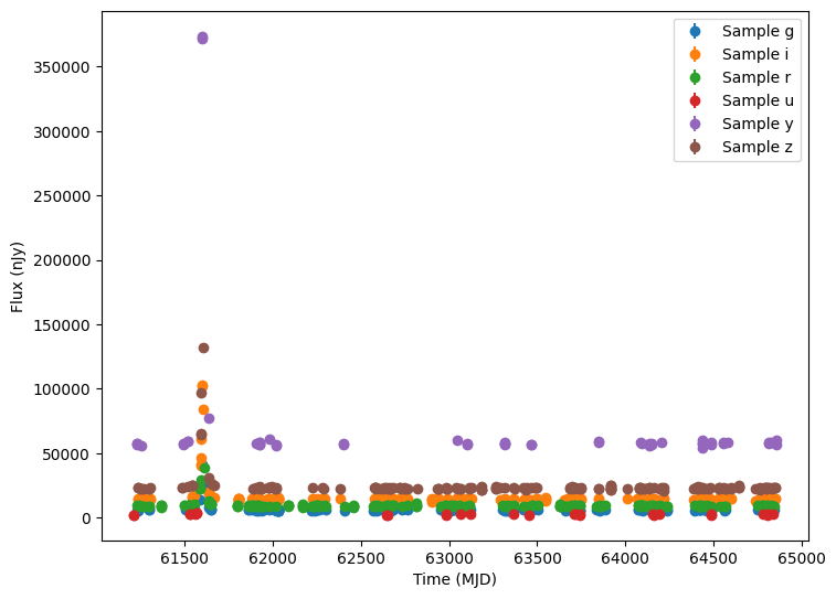
The good news is that the microlensing event shows up where expected (t0=61600). Unfortunately the bad news is that all three simulated events are identical, because we created the model using a fixed set of parameters. We just simulated the same microlensing event three times.

Adding LightCurveLynx Dynamic Sampling

We can make the LightCurveLynx wrapper more powerful by allowing the parameters to be set by the package’s sampling framework. As shown in other tutorial notebooks, parameters of a LightCurveLynx model can be set from a variety of sources, including constants or parameters from other nodes. In order to support a dynamic parameter, we use the add_parameter() function to add it to the model object. It will then be incorporated into the sampling flow.

Let’s start by modifying our model wrapper class to register and use each of the bagle model’s parameter. Since they are passed as a dictionary, we can iterate over the items in the dictionary.

class BagleModel(BandfluxModel):
    """A wrapper for a Bagle model with a flexible set of parameters."""

    # Convenience mapping from filter name to index in the parameter list.
    _filter_idx = {"u": 0, "g": 1, "r": 2, "i": 3, "z": 4, "y": 5}

    def __init__(self, model_name, parameter_dict, **kwargs):
        # We start by extracting the parameter information needed for a general physical model.
        ra = parameter_dict["raL"]
        dec = parameter_dict["decL"]
        t0 = parameter_dict["t0"]

        # Call the parent class constructor to set up the model.
        super().__init__(ra=ra, dec=dec, t0=t0, **kwargs)

        # Add all of the parameters in the dictionary as settable parameters (if they are not
        # already set by the parent class) and save their names (in order) for later use.
        self.parameter_names = []
        for param_name, param_value in parameter_dict.items():
            self.parameter_names.append(param_name)
            if param_name not in self.list_params():
                self.add_parameter(param_name, param_value)

        # Save the model name and class, but DO NOT create the model object yet.
        self.model_name = model_name
        self.model_class = getattr(model, model_name)

    def compute_bandflux(self, times, filter, state):
        """Evaluate the model at the passband level for a single, given graph state and filter.

        Parameters
        ----------
        times : numpy.ndarray
            A length T array of observer frame timestamps in MJD.
        filter : str
            The name of the filter.
        state : GraphState
            An object mapping graph parameters to their values with num_samples=1.
            This is not used in this model, but is required for the function signature.

        Returns
        -------
        bandflux : numpy.ndarray
            A length T array of band fluxes for this model in this filter.
        """
        # Extract the local parameters for this object from the full state object.
        local_params = self.get_local_params(state)

        # Create the bagle model object and set the parameters from the current state. We do this
        # here because the parameters saved in `state` will be different in each run.
        current_params = {param_name: local_params[param_name] for param_name in self.parameter_names}
        model_obj = self.model_class(**current_params)

        # Use the newly created model object with the current parameters to compute the photometry.
        mags = model_obj.get_photometry(times, self._filter_idx[filter])
        bandflux = mag2flux(mags)
        return bandflux

The Init Function

The __init__() function is similar to the earlier example. It starts by extracting the parameters needed by the base class (RA, dec, and t0) and calling that class’s constructor. Again the actual code we would want to use in production is a bit more complex because we also want to check kwargs for these values and bagle can use other parameters to compute t0. We keep the code simple here for illustration purposes. For a productionized version of this code see models/bagle_models.py, which handles several edge cases.

The init function then iterates through the given dictionary saving a list of all the keys and adding any unknown parameters to the model. Note that we need to check whether a parameter already exists because the t0 parameter may already be added by the base class’s constructor.

Unlike the previous implementation, this constructor does not create the object. As we will see next, this is because we need to create a new object for each set of parameters we have sampled.

The Compute Function

The compute_bandflux() extracts the sampled parameters from the state object and constructs a dictionary from them. The state object holds all the sampled parameter data for each run of the simulation, allowing users to replay all or part of the simulation. These objects are created when sampling the model’s parameters and their values filled in according to the recipes that define each parameter.

Once the function has constructed the dictionary object, it instantiates a new instance of the bagle model and uses it to generate the fluxes. While this might seem wasteful (we only use the object once), it is necessary because we need each of the objects to have different sets of parameters.

Modifying the Simulation

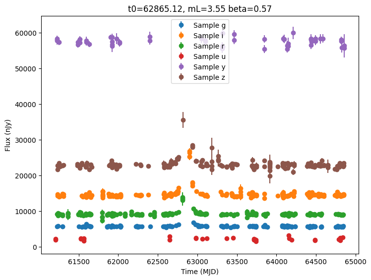
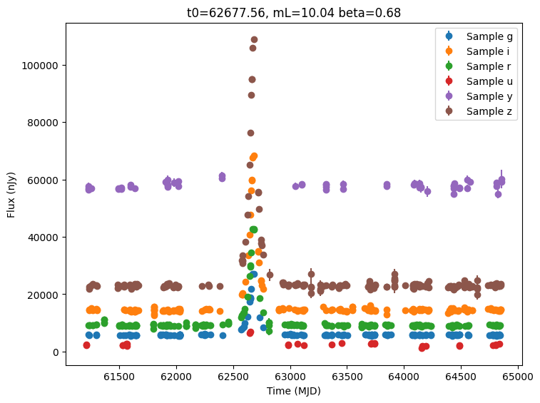
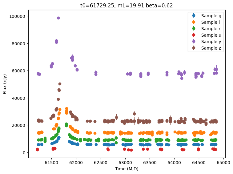
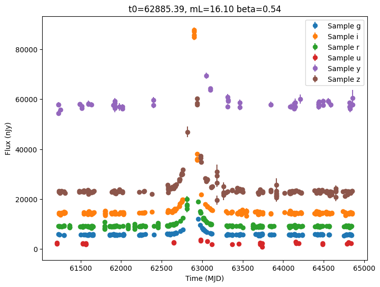
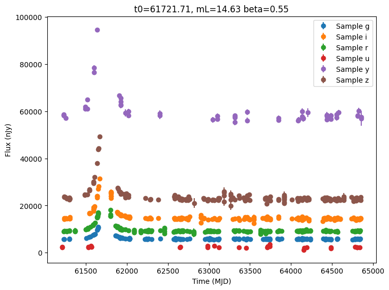
To use the newly supported settable parameters, let’s expand out the parameter dictionary so that three of the parameters are randomly chosen:

• mL will be sampled uniformly from [1,10) solar masses.

• t0 will be sampled uniformly from [61000, 63000)

• beta be sampled from a normal distribution with mean=0.6 and std=0.1.

from lightcurvelynx.math_nodes.np_random import NumpyRandomFunc

dL = 4000  # Distance to lens
dS = 8000  # Distance to source
parameter_dict2 = {
    "raL": 270.66679,
    "decL": -35.70483,
    "mL": NumpyRandomFunc("uniform", low=1, high=20),
    "t0": NumpyRandomFunc("uniform", low=61000, high=63000),
    "beta": NumpyRandomFunc("normal", loc=0.6, scale=0.1),
    "dL": dL,
    "dL_dS": dL / dS,
    "xS0_E": 0.0,  # arbitrary offset (arcsec)
    "xS0_N": 0.0,  # arbitrary offset (arcsec)
    "muL_E": 5.0,
    "muL_N": 10.0,
    "muS_E": 0.0,
    "muS_N": 0.0,
    "b_sff": [1, 1, 1, 1, 1, 1],
    "mag_src": [23, 22, 21.5, 21, 20.5, 19.5],
}

# Create the source object.
source2 = BagleModel(model_name, parameter_dict2)

Once again, we sample and simulate the new objects.

lightcurves = simulate_lightcurves(
    source2,
    5,
    survey_info,
    param_cols=["BagleModel_0.mL", "BagleModel_0.beta"],
)

for idx in range(5):
    # Extract the row for this object.
    lc = lightcurves.loc[idx]

    # Plot the lightcurves.
    ax = plot_lightcurves(
        fluxes=np.asarray(lc["lightcurve"]["flux"], dtype=float),
        times=np.asarray(lc["lightcurve"]["mjd"], dtype=float),
        fluxerrs=np.asarray(lc["lightcurve"]["fluxerr"], dtype=float),
        filters=np.asarray(lc["lightcurve"]["filter"], dtype=str),
        title=(f"t0={lc['t0']:.2f}, mL={lc['BagleModel_0_mL']:.2f} beta={lc['BagleModel_0_beta']:.2f}"),
    )
    ax.legend()
    plt.show()

Simulating: 100%|██████████| 5/5 [00:00<00:00, 202.75obj/s]

Presampled Values

If the user has their own sampling infrastructure, they might not be interested in using the random number generators provided by LightCurveLynx. In that case, we can still use the same approach in constructing our wrapper model, but change how the parameters are feed into the model.

Let’s consider the case where some of the model parameters are pre-sampled and provided as an astropy Table (note other data structures, such as a pandas DataFrame could also be used).

from astropy.table import Table

num_samples = 10

# Build a list of different mag_src values for each sample. Draw each
# list of magnitudes from a normal distribution around given mean values.
mag_list = []
mean_mags = np.array([23, 22, 21.5, 21, 20.5, 19.5])
for i in range(num_samples):
    mag_list.append(np.random.normal(mean_mags, 0.5))

param_table = Table(
    {
        "mL": [1.0, 2.0, 2.5, 3.0, 3.1, 4.0, 5.0, 6.0, 7.0, 8.0],
        "t0": [61510, 61520, 61530, 61540, 61550, 61560, 61570, 61580, 61590, 61600],
        "beta": [0.2, 0.3, 0.4, 0.5, 0.6, 0.7, 0.8, 0.9, 1.0, 1.1],
        "xS0_E": np.random.normal(0.0, 0.1, num_samples).tolist(),
        "xS0_N": np.random.normal(0.0, 0.1, num_samples).tolist(),
        "mag_src": mag_list,
    }
)
print(param_table)

 mL   t0  ...         xS0_N                         mag_src
--- ----- ... --------------------- ----------------------------------------
1.0 61510 ...  -0.03892934503319601  22.848264869049775 .. 18.82724609818703
2.0 61520 ... -0.025881655540215365 23.662292535590392 .. 18.215094149783265
2.5 61530 ...   0.05696236288896426 23.081924307613317 .. 18.850430728710972
3.0 61540 ...    -0.092717412490678 22.652254723449218 .. 19.780762172683712
3.1 61550 ...  -0.12507576986078298 22.435201609322043 .. 20.608689914464343
4.0 61560 ...  0.016749964921144927   22.71556848069735 .. 18.48234395270818
5.0 61570 ... -0.009341002682468217  22.394748758899027 .. 19.22961401547571
6.0 61580 ...   -0.0148871524169763  22.75670841727394 .. 18.865753325086366
7.0 61590 ...   0.04627700081497887 22.728813817303248 .. 19.345197106372378
8.0 61600 ...  -0.13471447346498797  22.520045822167532 .. 19.50137021451929

We can use the TableSampler class provided in the math_nodes/given_sampler.py which reads paramters out of a table. By setting in_order=True the rows will be used in-order. Otherwise the values will be randomly sampled. NOTE: The TableSamplerdoes not support in-order traversal when performing distributed computation.

Users can access the parameters from the table sampler using the dot notation with the parameter name.

from lightcurvelynx.math_nodes.given_sampler import TableSampler

table_sampler = TableSampler(param_table, in_order=False)

parameter_dict2 = {
    "raL": 270.66679,  # Constant RA
    "decL": -35.70483,  # Constant Dec
    "mL": table_sampler.mL,  # The mL values from the table (in order)
    "t0": table_sampler.t0,  # The t0 values from the table (in order)
    "beta": table_sampler.beta,  # The beta values from the table (in order)
    "dL": dL,  # Constant dL
    "dL_dS": dL / dS,  # Constant dL/dS
    "xS0_E": table_sampler.xS0_E,  # The xS0_E values from the table (in order)
    "xS0_N": table_sampler.xS0_N,  # The xS0_N values from the table (in order)
    "muL_E": 5.0,  # Constant muL_E
    "muL_N": 10.0,  # Constant muL_N
    "muS_E": 0.0,  # Constant muS_E
    "muS_N": 0.0,  # Constant muS_N
    "b_sff": [1, 1, 1, 1, 1, 1],
    "mag_src": table_sampler.mag_src,  # A different mag_src list for each sample
}

# Create the source object.
source3 = BagleModel(model_name, parameter_dict2)

When we run the simulation, the values used to create the bagle models will be a combination of the constant values and the values from the table. The TableSampler ensures that the same row is used for all the parameters in a sample, so they are consistent.

We can print some of these values from the results to see what the simulation looks like.

lightcurves = simulate_lightcurves(source3, 10, survey_info, param_cols=["BagleModel_0.mL"])

for idx in range(10):
    row = lightcurves.loc[idx]
    print(f"{idx}: ({row['ra']}, {row['dec']}): t0={row['t0']}, mL={row['BagleModel_0_mL']}")

Simulating: 100%|██████████| 10/10 [00:00<00:00, 214.25obj/s]

0: (270.66679, -35.70483): t0=61520, mL=2.0
1: (270.66679, -35.70483): t0=61570, mL=5.0
2: (270.66679, -35.70483): t0=61550, mL=3.1
3: (270.66679, -35.70483): t0=61590, mL=7.0
4: (270.66679, -35.70483): t0=61550, mL=3.1
5: (270.66679, -35.70483): t0=61570, mL=5.0
6: (270.66679, -35.70483): t0=61540, mL=3.0
7: (270.66679, -35.70483): t0=61510, mL=1.0
8: (270.66679, -35.70483): t0=61540, mL=3.0
9: (270.66679, -35.70483): t0=61510, mL=1.0

Conclusion

This notebook shows how we can create a basic wrapper for the bagle models. A full featured version can be found in models/bagle_models.py, including:

• The ability to set a custom filter map.

• Conditional imports for the bagle package.

• Various helper functions.