Time Varying EffectModels

The impact of an EffectModel can vary with time and wavelength (or filter). In this notebook, we show how to construct a basic time varying effect model.

In this notebook we model a Gaussian activation function, such as we might see if the contribution of an object to the observed flux followed a Gaussian curve over time. For example we might have a high proper motion star whose contribution to the current field of view varies with time and PSF as it moves into and then out of the field of view. The percentage of its flux is determined by the Gaussian smearing of the PSF.

import numpy as np
import matplotlib.pyplot as plt

from lightcurvelynx.effects.effect_model import EffectModel
from lightcurvelynx.models.basic_models import ConstantSEDModel

/home/docs/checkouts/readthedocs.org/user_builds/lightcurvelynx/envs/stable/lib/python3.12/site-packages/tqdm/auto.py:21: TqdmWarning: IProgress not found. Please update jupyter and ipywidgets. See https://ipywidgets.readthedocs.io/en/stable/user_install.html
  from .autonotebook import tqdm as notebook_tqdm

We start be defining our new effect model. Below we only show the implementation for apply() which applies the effects to the SED. The code for apply_bandflux() would be almost identical. Our new model inherits from the base effect model.

class GaussianActivation(EffectModel):
    """An effect that applies a Gaussian multiplier to the flux density.
    This is primarily included as a demonstration of how to implement effects
    that vary with time, but could be used to model a fast moving star that
    moves through the field of view.

    flux = flux * exp(-0.5 * ((time - t0) / decay) ** 2)

    Attributes
    ----------
    t0 : parameter
        The peak time of the effect (in days).
    decay : parameter
        The decay time of the effect (in days).
    rest_frame : bool
        Whether the effect is applied in the rest frame of the observation (True)
        or in the observed frame (False).
    """

    def __init__(self, t0, decay, rest_frame=True, **kwargs):
        super().__init__(**kwargs)

        # Define the effect's parameters. Note that these do not need to match
        # the argument names. They should be chosen so that they do not overlap
        # parameters within the model node (e.g. we can't use t0).
        self.add_effect_parameter("gaussian_activation_t0", t0)
        self.add_effect_parameter("gaussian_activation_decay", decay)

        # Set the rest_frame parameter.
        self.rest_frame = rest_frame

    def apply(
        self,
        flux_density,
        times=None,
        wavelengths=None,
        gaussian_activation_t0=None,
        gaussian_activation_decay=None,
        **kwargs,
    ):
        """Apply the effect to observations (flux_density values).

        Parameters
        ----------
        flux_density : numpy.ndarray
            A length T X N matrix of flux density values (in nJy).
        times : numpy.ndarray, optional
            A length T array of times (in MJD). Not used for this effect.
        wavelengths : numpy.ndarray, optional
            A length N array of wavelengths (in angstroms). Not used for this effect.
        gaussian_activation_t0 : float, optional
            The peak time of the effect (in days). Raises an error if None is provided.
        gaussian_activation_decay : float, optional
            The decay time of the effect (in days). Raises an error if None is provided.
        **kwargs : `dict`, optional
           Any additional keyword arguments, including any additional
           parameters needed to apply the effect.

        Returns
        -------
        flux_density : numpy.ndarray
            A length T x N matrix of flux densities after the effect is applied (in nJy).
        """
        # Basic error checking to make sure we got values for the parameters we need.
        if gaussian_activation_t0 is None or gaussian_activation_decay is None:
            raise ValueError("gaussian_activation_t0 and gaussian_activation_decay must be provided")
        if times is None:
            raise ValueError("times must be provided")

        # Compute the scale at each time and apply it.
        scale = np.exp(-0.5 * ((times - gaussian_activation_t0) / gaussian_activation_decay) ** 2)
        return flux_density * scale[:, np.newaxis]

Now that we have an effect model, we can create a model object and apply the effect.

model = ConstantSEDModel(brightness=100.0)
model.add_effect(GaussianActivation(t0=5.0, decay=2.0))

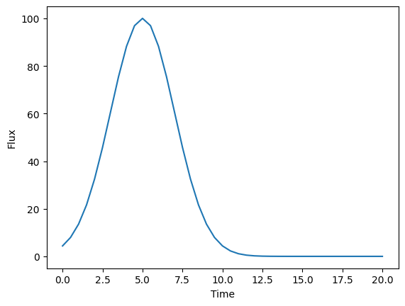
We then run a simulation on this object and plot the flux density at the first wavelength over our time range.

times = np.arange(0.0, 20.5, 0.5)
wavelengths = np.array([1000.0, 2000.0, 3000.0, 4000.0])
flux_density = model.evaluate_sed(times=times, wavelengths=wavelengths)

# Plot the first wavelength's flux density over time
plt.plot(times, flux_density[:, 0])
plt.xlabel("Time")
plt.ylabel("Flux")
plt.show()

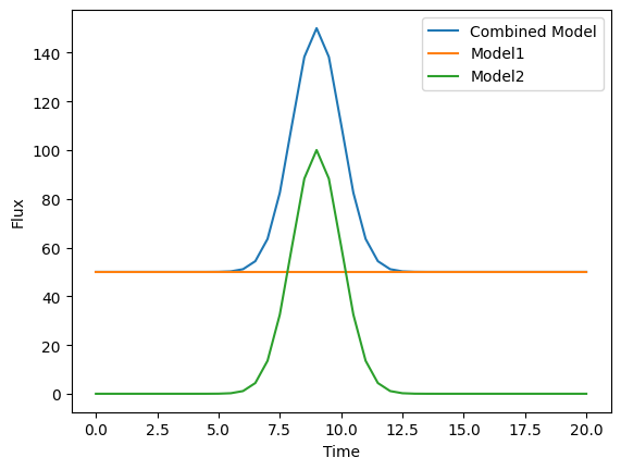
We can make the simulation more realistic by defining a compound object and applying this activation to only one of the sources.

from lightcurvelynx.models.multi_object_model import AdditiveMultiObjectModel

model1 = ConstantSEDModel(brightness=50.0)

model2 = ConstantSEDModel(brightness=100.0)
model2.add_effect(GaussianActivation(t0=9.0, decay=1.0))

combined_model = AdditiveMultiObjectModel([model1, model2])

# Evaluate the combined model at different times.
wavelengths = np.array([4000.0])
fluxes1 = model1.evaluate_sed(times, wavelengths)
fluxes2 = model2.evaluate_sed(times, wavelengths)
fluxes_all = combined_model.evaluate_sed(times, wavelengths)

plt.plot(times, fluxes_all, label="Combined Model")
plt.plot(times, fluxes1, label="Model1")
plt.plot(times, fluxes2, label="Model2")
plt.xlabel("Time")
plt.ylabel("Flux")
plt.legend()
plt.show()