Custom Surveys

This notebook demonstrates how to support a new survey by creating a custom ObsTable subclass. By creating your survey as a subclass of ObsTable, you will inherit almost all the functionality needed to use the survey in a simulation (as well as numerous helper functions). We discuss what information you will need to provide, which functions you need to create, and how you can use the new survey.

Survey Data

LightCurveLynx requires a few different pieces of information from the survey:

where the survey is looking (time, RA, dec, fov)
the noise characteristics of the observations (zero point, magnitude limit)
the information about the filters and their transmission curves

This data can come from a simulation or a real survey.

ObsTable

ObsTable (short for Observation Table) is the foundational object for storing information about a survey’s pointings and noise characteristics. It can generally be viewed as a table with a single row for each image exposure. Internally this per-observation data is stored in a Pandas data frame called _table. At a minimum the table requires columns for time (in MJD), RA (in degrees), and dec (in degrees). Many surveys include a lot of other data in this table, such as the filter used for the observation and the seeing at the time of the observation.

The ObsTable object also stores survey-wide values in a dictionary called survey_values. This data includes core survey information such as the radius of the field of view in degrees (called radius), which is needed for spatial matching. It also includes all of the constants used in computing noise values, such as the detector’s dark current values and the pixel scale. The exact values tracked will vary from survey to survey. The only required one is a radius.

Example

For concreteness, let’s consider the ObsTable for one of the fake data sets included in the test data. This data is in the Rubin OpSim format, so we load it with the OpSim subclass of ObsTable.

[1]:

from lightcurvelynx.obstable.opsim import OpSim

# Load the OpSim data from a local database file.
opsim = OpSim.from_db("../../tests/lightcurvelynx/data/opsim_small.db")
print(f"Loaded OpSim with {len(opsim)} rows.")

print("\nSurvey Constants:")
for key, value in opsim.survey_values.items():
    print(f"  {key}: {value}")

print("\nFirst 5 rows of the OpSim table:")
opsim._table.head()

Loaded OpSim with 300 rows.

Survey Constants:
  ccd_pixel_width: 4000
  ccd_pixel_height: 4000
  dark_current: 0.2
  ext_coeff: {'u': -0.458, 'g': -0.208, 'r': -0.122, 'i': -0.074, 'z': -0.057, 'y': -0.095}
  nexposure: 1
  pixel_scale: 0.2
  radius: 1.75
  read_noise: 8.8
  zp_per_sec: {'u': 26.524, 'g': 28.508, 'r': 28.361, 'i': 28.171, 'z': 27.782, 'y': 26.818}
  zp_err_mag: 0.0001
  survey_name: LSST

First 5 rows of the OpSim table:

/home/docs/checkouts/readthedocs.org/user_builds/lightcurvelynx/envs/stable/lib/python3.12/site-packages/tqdm/auto.py:21: TqdmWarning: IProgress not found. Please update jupyter and ipywidgets. See https://ipywidgets.readthedocs.io/en/stable/user_install.html
  from .autonotebook import tqdm as notebook_tqdm

[1]:

	index	time	dec	observationId	filter	exptime	nexposure	airmass	seeing	seeingFwhmGeom	skybrightness	zp	psf_footprint	sky_bg_e
0	0	60676.000	-30.0	0	g	29.2	2	1.3	1.12	0.97	20.0	0.520448	71.067407	2790.505243
1	1	60676.003	-27.0	1	g	29.2	2	1.3	1.12	0.97	20.0	0.520448	71.067407	2790.505243
2	2	60676.006	-24.0	2	g	29.2	2	1.3	1.12	0.97	20.0	0.520448	71.067407	2790.505243
3	3	60676.009	-21.0	3	g	29.2	2	1.3	1.12	0.97	20.0	0.520448	71.067407	2790.505243
4	4	60676.012	-18.0	4	g	29.2	2	1.3	1.12	0.97	20.0	0.520448	71.067407	2790.505243

Data from either the survey values or the survey table can be accessed using the [] notation. If the data is pulled from the table it will be returned as a Pandas series. If it comes from the survey values it will be whatever type was used to set it (int, float, list, etc.)

[2]:

# Access a constant value for the survey.
print("ccd_pixel_width: ", opsim["ccd_pixel_width"])

# Access the table values for a specific column.
print("\nRA values: ", opsim["ra"])

ccd_pixel_width:  4000

RA values:  0       0.0
1       0.0
2       0.0
3       0.0
4       0.0
       ...
295    27.0
296    27.0
297    27.0
298    27.0
299    27.0
Name: ra, Length: 300, dtype: float64

Pointing Information

As noted above, the survey’s pointing information must be provided by three columns with predefined names time, ra, and dec with units of days, degrees, and degrees respectively. This information, along with either the fov’s radius or the detector footprint, are used to determine the times at which a give object is observed.

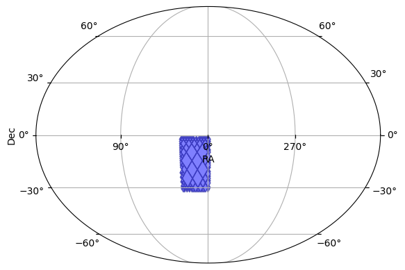
We can also use it to estimate coverage of the survey or plot the overall footprint.

[3]:

opsim.plot_footprint()

[3]:

(<Figure size 640x480 with 1 Axes>, <WCSAxes: >)

../_images/notebooks_custom_survey_6_1.png

Creating a New Survey Type

There are only a few functions and parameters that need to be set to create a new ObsTable subclass. We first describe these below and then present an example code block.

Constructor

At a minimum, the __init__ function needs to take the Pandas table of input values and pass it along to the parent class’s constructor. It can also be used to preprocess the data, such as converting units or setting up mappings of filter names to saturation values.

The preprocessing step of renaming columns is common enough that it is supported in the ObsTable constructor directly. You can provide the constructor a column map, which automatically renames the table’s columns to match what is expected by your code. The map is a directionally where each key indicates the final column name and its value can either be a string (given name) or list of strings (list of possible names) in the data. For example if the column map is {"ra": ["fieldRA", "osbRA"]}, the code will check the input table either “fieldRA” or “obsRA” and rename that column to “ra”. If there are multiple matches, only the first will be used.

Survey Values

The ObsTable class uses a _default_survey_values class attribute to provide the default survey constants, such as “dark_current”, “pixel_scale”, or “radius”. The attribute is a dictionary mapping the information’s name to its value. The subclass can define its own _default_survey_values dictionary with its corresponding values. The only survey value that is required if the radius of the camera’s field of view (radius).

We also recommend including the survey_name so you can track information. This name can be used to match the survey to default passbands or noise models (if not already specified).

We highly recommend including the units in a comment after each parameter.

Noise Computation

The information about the observation’s noise characteristics varies per-survey, so the ObsTable class relies on a helper functions: _derive_noise_columns(self) that computes any derived columns that are needed for noise computation. For example, most tables and noise models will need the zero points for each row in nJy (which produces 1 e-) appended as an column called zp. If the table already contains the values needed, it should skip the computation.

ExampleObsTable

Let’s now create an example ObsTable subclass. We add description through the comments instead of breaking up the code block.

[4]:

from lightcurvelynx.astro_utils.mag_flux import mag2flux
from lightcurvelynx.obstable.obs_table import ObsTable


class ExampleObsTable(ObsTable):
    """An example ObsTable subclass."""

    # Default survey values (using numbers for LSSTCam). Each of these is a map
    # from information name to its value for the entire survey.
    _default_survey_values = {
        "dark_current": 0.022,  # electrons per second per pixel
        "gain": 1.595,  # electrons per ADU
        "pixel_scale": 0.2,  # arcsec/pixel
        "radius": 1.75,  # degrees
        "read_noise": 5.82,  # readout electrons per pixel
        "survey_name": "my_awesome_survey",
    }

    # A column mapping to use for this survey. This allows us to support
    # reading from different data formats without writing new classes.
    _default_colmap = {
        "filter": "band",  # Map band->filter
    }

    # The constructor
    def __init__(self, table, colmap=None, **kwargs):
        # Set the default column map is none is provided.
        colmap = self._default_colmap if colmap is None else colmap

        # Call the parent constructor to initialize the table, spatial data structures, etc.
        super().__init__(table, colmap=colmap, **kwargs)

    def _derive_noise_columns(self):
        """Pre-compute the zero points (in nJy) for each observation using whatever data
        your custom survey has. This function is optional if your code does not use zeropoints
        in the noise model.
        """
        if "zp" in self._table.columns:
            return  # Nothing to do. We already have a "zp" column.

        # Let's assume our custom survey provides the zero points as magnitudes as "zp_mag_e"
        # for the electron-based zero point (as a magnitude). We convert it to nJy and add it
        # back as a column.
        if "zp_mag_e" in self._table.columns:
            zp_values = mag2flux(self._table["zp_mag_e"])
            self.add_column("zp", zp_values, overwrite=True)
            return

        # Since we will need zero point for the noise model below, we throw an error
        # if we don't have enough information to compute it.
        raise ValueError("Not enough information to compute the zero points.")

In addition, users can create a custom FluxNoiseModel subclass if they want to use a different noise model for this survey.

In this example, we will define a new subclass of the builtin PoissonFluxNoiseModel that fixes some of the survey constants and specifies matching column names. Alternatively we could build our custom survey with the standard fields required by the base PoissonFluxNoiseModel or use a different noise model such as ConstantFluxNoiseModel.

[5]:

from lightcurvelynx.noise_models.base_noise_models import PoissonFluxNoiseModel
from lightcurvelynx.noise_models.noise_utils import poisson_bandflux_std


class ExampleNoiseModel(PoissonFluxNoiseModel):
    """A subclass of PoissonFluxNoiseModel for Example survey data."""

    # These are values that the noise model needs to read from the ObsTable.
    _required_values = ["sky_bg_e", "zp", "read_noise", "dark_current"]

    def __init__(self):
        super().__init__()

    def compute_flux_error(self, bandflux, obs_table, indices):
        """Compute the flux error for the given bandflux and observation parameters.

        Parameters
        ----------
        bandflux : array_like of float
            Source bandflux in energy units, e.g. nJy.
        obs_table : ObsTable
            Table containing the observation parameters, including all
            parameters needed to compute the noise.
        indices : array_like of int
            Indices of the observations in the ObsTable for which to compute the noise.

        Returns
        -------
        flux_err : array_like
            The standard deviation of the bandflux measurement error, in the
            same units as the input bandflux.
        """
        # For simplicity, we use the built-in Poisson noise model with some constants.
        # The function uses a mixture of per-row data (such as zeropoint) and survey-wide
        # constants (such as read noise and dark current) to compute the noise.
        # Users can implement their own functions to reflect the survey's characteristics.
        return poisson_bandflux_std(
            bandflux,
            total_exposure_time=30.0,  # Constant exposure time.
            exposure_count=1,  # Single exposure.
            psf_footprint=10.0,  # PSF footprint in arcsec^2.
            sky=obs_table["sky_bg_e"].iloc[indices],  # sky background in e- from each row
            zp=obs_table["zp"].iloc[indices],  # zero point in nJy from each row
            readout_noise=obs_table.safe_get_survey_value("read_noise"),  # Survey-wide constant
            dark_current=obs_table.safe_get_survey_value("dark_current"),  # Survey-wide constant
            zp_err_mag=0.01,  # Use a constant noise floor for example.
        )

We can create a fake ObsTable from a table of given values.

[6]:

import pandas as pd

table_data = {
    "time": [60676.0, 60676.1, 60676.2],
    "ra": [10.0, 20.0, 10.0],
    "dec": [-10.0, -20.0, -10.0],
    "band": ["r", "r", "r"],
    "zp_mag_e": [25.0, 25.5, 26.0],  # Zero point magnitudes for the example.
    "sky_bg_e": [100.0, 150.0, 200.0],  # Sky background in electrons for the example.
}
pdf = pd.DataFrame(table_data)

obs_table = ExampleObsTable(pdf, noise_model=ExampleNoiseModel())
obs_table.head()

[6]:

	time	ra	dec	filter	zp_mag_e	sky_bg_e	zp
0	60676.0	10.0	-10.0	r	25.0	100.0	363.078055
1	60676.1	20.0	-20.0	r	25.5	150.0	229.086765
2	60676.2	10.0	-10.0	r	26.0	200.0	144.543977

As you can see from the displayed table, the columns have been renamed according to the column map (band->filter) and the zero point column has automatically been added by the _derive_noise_columns() function.

Using Tables in Simulations

The new ObsTable subclass can be used in a simulation like any other table. To run the simulation, we also need a model of the source and the transmission curves for the survey’s passband.

NOTE: Although filter transmission curves are part of the survey information, we break them out into their own object (PassbandGroup) to allow separate analysis. If your survey uses different filters, you will need to load them as well. See the Passband Demo notebook for details on loading new passbands.

We start be loading the passbands that we will use. In this example, we use the passbands from LSST (but use a cached local version in the test directory to avoid a download).

[7]:

from lightcurvelynx.astro_utils.passbands import PassbandGroup

table_dir = "../../tests/lightcurvelynx/data/passbands"
passband_group = PassbandGroup.from_preset(preset="LSST", table_dir=table_dir)

Then we define a simple sin wave model for the simulation. We choose the position (RA, dec) to match two of the three observations in our fake table.

[8]:

from lightcurvelynx.models.basic_models import SinWaveModel

source = SinWaveModel(
    brightness=1e16,
    amplitude=2e15,
    frequency=11.0,
    ra=10.0,
    dec=-10.0,
    t0=0.0,
    node_label="sin_wave_source",
)

Then we run the simulation and look at the resulting light curve for our single simulated object.

[9]:

from lightcurvelynx.simulate import simulate_lightcurves
from lightcurvelynx.survey_info import SurveyInfo

survey_info = SurveyInfo(
    obstable=obs_table,
    passbands=passband_group,
    noise_model=ExampleNoiseModel(),
)
results = simulate_lightcurves(source, 1, survey_info)
lightcurve = results.iloc[0]["lightcurve"]
lightcurve

Simulating: 100%|██████████| 1/1 [00:00<00:00, 382.66obj/s]

[9]:

	mjd	filter	flux	fluxerr	flux_perfect	survey_idx	obs_idx	is_saturated
0	60676.0	r	9.886567e+15	9.210340e+13	1.000000e+16	0	0	False
1	60676.2	r	1.176736e+16	1.096225e+14	1.190211e+16	0	2	False

As we can see from the light curve table, the object is observed at the correct two times (MJD 60676.0 and 60676.2) with different pre-noise fluxes (flux_perfect) corresponding to different points on the sin wave. Each observation also has added noise based on the survey’s characteristics and input data.

Warnings and Caveats

The most common problems we encounter when creating a new survey type are understanding the survey’s columns and ensuring the correct units. For example, consider a column named sky_bg that holds the sky background. Even given this knowledge, the we do not have enough information. Is the background value given in electron, ADU, or something else? We recommend thoroughly validating the output produced by each new survey to ensure accuracy.