Introduction
LightCurveLynx is a package for large-scale, time-domain forward-modeling of astronomical light curve data. Simulations incorporate realistic effects, including survey cadence, dust extinction, and instrument noise models. LightCurveLynx is designed to enable user extensibility, such as adding new models, effects, and instruments, while ensuring scalability.
In this tutorial, we discuss the overall flow of LightCurveLynx and how to use it to run simulations. The goal is to get a new user started and allow them to explore the package.
Later tutorials cover topics in more depth, including:
Sampling Parameters (sampling.ipynb) - Provides an introduction to parameters and how they are sampled within a simulation run.
Adding new model types (adding_models.ipynb) - Provides a more in-depth discussion of
BasePhysicalModel,BandfluxModel, andSEDModelsubclasses and how to add new models.Add new effect types (addings_effects.ipynb) - Provides a discussion of the
EffectModelclass, how it is used, and how to create new subclasses.Working directly with passbands (passband-demo.ipynb)
Working directly with ObsTables / Rubin OpSims (opsim_notebook.ipynb)
Program Flow
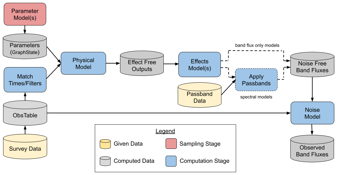
LightCurveLynx generates synthetic light curves using the stages shown in the illustration below. A BasePhysicalModel and information about the parameter distributions is used to sample the models. These are combined with information from an ObsTable, such as a Rubin OpSim, to generate sample flux densities at a given set of times and wavelengths (or passbands), accounting for effects such as redshift. The simulator also applies other relevant effects to the rest frame flux densities
(e.g. dust extinction) and the observer frame flux densities (e.g. detector noise). At the end the code outputs a series of samples.
A user has several important questions to answer when doing a new simulation:
What do you want to simulate (supernova, kilanova, AGN, etc.)? The answer to this question determines the subclass of
BasePhysicalModelyou will use to create the model object. For example, if you want to simulate a kilanova using theredbackpackage, you would start by creatingRedbackWrapperModelobject. If you want to use a SALT2 supernova model, you may start with theSncosmoWrapperModel.What parameters does your model have? And how do you want to set them? The answers to these questions determine how you set the parameters of the model object. All parameters within a model are set using arguments in the object’s constructors.
What effects do you want to apply to the light coming from this object? The answer to this question will determine which effect objects you create and add to the object.
Under what conditions do you want to observe this object? What is your viewing cadence and instrument noise characteristics? In short, what
SurveyInfo(ObsTable,PassbandGroup, and noise model) are you using? Most users will just need to choose from one of the predefined survey options, such as LSST or ZTF.
[1]:
# Display logging warning messages to the console to help track progress.
# This is optional but useful for long-running simulations.

import logging

logging.basicConfig(level=logging.WARNING)
Models
All light curves are generated from model objects that are a subclass of the BasePhysicalModel class. These model objects provide mechanisms for:
Sampling their parameters from given distributions,
Generating flux densities at given times and wavelengths (or passbands), and
Applying noise and other effects to the observations.
All of these steps are performed behind the scenes, so a user only needs to know what type of object they are simulating and select the corresponding class.
A major goal of LightCurveLynx is to be easily extensible so that users can warp existing packages or entirely new models. See the adding_models.ipynb notebook for examples of how to add a new type of models. For examples of wrapping models see the Wrapping BAGLE Models, Wrapping Redback Models, or Wrapping VBMicroLensing notebooks.
Samples
Each “sample” of the data corresponds to output from a single simulated source. This output is created by first sampling the model’s parameter (creating a well-defined source) and then using those parameters to generate the output flux. When a user generates a hundred samples, they are generating 100 light curves from 100 sample astronomical sources. For a detailed description of how parameter sampling works, see the sampling.ipynb notebook.
We can demonstrate this simulation flow using SinWaveModel, a toy model that generates fluxes using a sin wave. The SinWaveModel object uses multiple parameters to generate its flux, so we need to specify how to set these. For some parameters we may have a fixed value, such as a brightness of 100.0.
Setting and Sampling Parameters
But in most simulations we will want the values of the parameters themselves to vary from source to source. We can set these from other nodes (any object that generates or uses parameters). Below we use the NumpyRandomFunc, one of LightCurveLynx’s built-in samplers, to set four of the parameters. We set two of the model’s parameters (frequency and t0) from uniform distributions. And we set two parameters (RA and dec) from a Gaussian that matches the toy survey information we
will load later in this notebook.
[2]:
from lightcurvelynx.math_nodes.np_random import NumpyRandomFunc
from lightcurvelynx.models.basic_models import SinWaveModel

model = SinWaveModel(
    brightness=2000.0,
    amplitude=200.0,
    frequency=NumpyRandomFunc("uniform", low=0.01, high=0.1),
    t0=NumpyRandomFunc("uniform", low=0.0, high=10.0),
    ra=NumpyRandomFunc("normal", loc=200.5, scale=0.01),
    dec=NumpyRandomFunc("normal", loc=-50.0, scale=0.01),
    node_label="sin_wave_model",
)
/home/docs/checkouts/readthedocs.org/user_builds/lightcurvelynx/envs/stable/lib/python3.12/site-packages/tqdm/auto.py:21: TqdmWarning: IProgress not found. Please update jupyter and ipywidgets. See https://ipywidgets.readthedocs.io/en/stable/user_install.html
  from .autonotebook import tqdm as notebook_tqdm
LightCurveLynx provides a range of tools for generating parameter values from a range of models and distributions. For example, we can sample the object’s position (RA, dec) directly from the survey data itself. For more information on how to define the parameter settings, see the sampling.ipynb notebook. For specific information on sampling (RA, dec), see the sampling_positions.ipynb notebook.
Generating Flux Densities
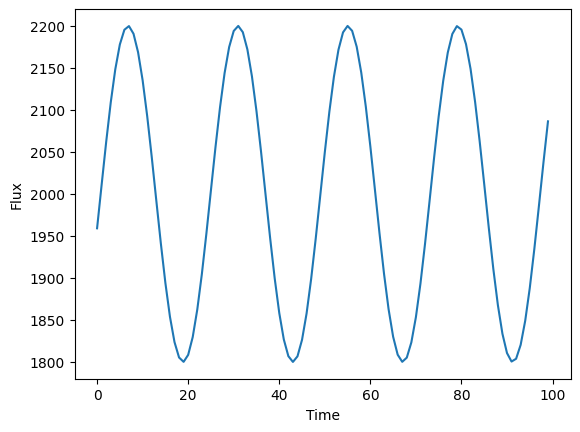
Once we have defined how the model’s parameters are set, we can use it to generate flux densities from the sampled input parameter values. We can manually evalute a model using the evaluate_sed() function where we provide the wavelengths and times to sample:
[3]:
import matplotlib.pyplot as plt
import numpy as np

times = np.arange(100.0)
wavelengths = np.array([7000.0])
fluxes = model.evaluate_sed(times, wavelengths)

plt.plot(times, fluxes)
plt.xlabel("Time")
plt.ylabel("Flux")
plt.show()
The power of the simulation software is that we can generate a large number of light curves from a distribution of models. We start by using a BasePhysicalModel object’s sample_parameters function to sample the parameters that can create this distribution of objects.
The GraphState Object
Let’s start with generating 5 sample objects. We save the samples in a GraphState object.
[4]:
state = model.sample_parameters(num_samples=3)
print(state)
NumpyRandomFunc:normal_1:
    loc: [200.5 200.5 200.5]
    scale: [0.01 0.01 0.01]
    function_node_result: [200.50914678 200.50695778 200.52085327]
sin_wave_model:
    ra: [200.50914678 200.50695778 200.52085327]
    dec: [-49.99157657 -49.99980078 -50.00269892]
    redshift: [None None None]
    t0: [9.20957128 9.66290224 3.59490722]
    distance: [None None None]
    brightness: [2000. 2000. 2000.]
    amplitude: [200. 200. 200.]
    frequency: [0.05016301 0.01290847 0.07906586]
NumpyRandomFunc:normal_2:
    loc: [-50. -50. -50.]
    scale: [0.01 0.01 0.01]
    function_node_result: [-49.99157657 -49.99980078 -50.00269892]
NumpyRandomFunc:uniform_3:
    low: [0. 0. 0.]
    high: [10. 10. 10.]
    function_node_result: [9.20957128 9.66290224 3.59490722]
NumpyRandomFunc:uniform_4:
    low: [0.01 0.01 0.01]
    high: [0.1 0.1 0.1]
    function_node_result: [0.05016301 0.01290847 0.07906586]
Most users will not need to interact directly with the GraphState object, but at a very high level it can be viewed as a nested dictionary where parameters are indexed by two levels. First, a node label tells the code which Python object is storing the parameter. This level of identification is necessary to allow different stages to use parameters with the same name. Second, the parameter name maps to its stored values.
Each (node name, parameter name) combination corresponds to a list of sample values for that parameter. Parameters are sampled together so that the i-th entires of each parameter represent a single, mutually consistent sampling of parameter space. For example, you may want to generate all the parameters for a Type Ia supernova given information about the host galaxy. For a lot more detail see the GraphState section in the sampling.ipynb
notebook. For now it is sufficient to know that state is an object tracking the sampled parameters’ values.
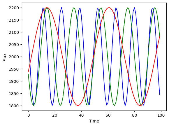
By passing the sampled state into evaluate_sed() we can generate multiple light curves (one for each sample) at once:
[5]:
fluxes = model.evaluate_sed(times, wavelengths, state)

plt.plot(times, fluxes[0, :], color="blue")
plt.plot(times, fluxes[1, :], color="green")
plt.plot(times, fluxes[2, :], color="red")
plt.xlabel("Time")
plt.ylabel("Flux")
plt.show()
Effects
Users can add effects to their physical model objects to account for real world aspects such as noise and dust extinction. For more detail on effects, including how to define your own, see the adding_effects.ipynb notebook.
Note: Detector noise and redshift are not added effects, but rather automatically applied. Redshift effects are applied to SED-type models only based on the object’s redshift parameter. Detector noise is applied to all model types from the ObsTable information (see the ObsTable section below for more details).
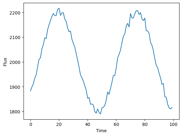
For this demo, we add a simple white noise effect to the model (rest frame). For real simulations we would want to add a range of effects, such as dust extinction.
[6]:
from lightcurvelynx.effects.white_noise import WhiteNoise

# Create the white noise effect.
white_noise = WhiteNoise(white_noise_sigma=10.0)
model.add_effect(white_noise)

# Evaluate the model with white noise applied (a single sample).
flux = model.evaluate_sed(times, wavelengths)
plt.plot(times, flux)
plt.xlabel("Time")
plt.ylabel("Flux")
plt.show()
ObsTable and Passbands
To generate a reasonable simulation we need to provide instrument, survey information, and noise model information. We use several classes (e.g., ObsTable and PassbandGroup) to work with this data and store the combination in a SurveyInfo object.
OpSim
The ObsTable object is used to store survey information, including pointings and weather conditions. In this notebook we use a specific subclass, OpSim, which models Rubin’s simulated operations database. For more detail on the OpSim class, its capabilities, and how to work with it, see the opsim_notebook.ipynb notebook.
The OpSim class is also used to extract information about the detector for modeling detector noise.
For this demo we load a small example database included with the code.
[7]:
from lightcurvelynx.obstable.opsim import OpSim

opsim_file = "../../tests/lightcurvelynx/data/opsim_shorten.db"
ops_data = OpSim.from_db(opsim_file)

print(f"Loaded an opsim database with {len(ops_data)} entries.")
print(f"Columns: {ops_data.columns}")
print(f"Time range: [{ops_data['time'].min()}, {ops_data['time'].max()}]")
Loaded an opsim database with 100 entries.
Columns: Index(['observationId', 'ra', 'dec', 'time', 'flush_by_mjd', 'exptime', 'band',
       'filter', 'rotation', 'rotSkyPos_desired', 'nexposure', 'airmass',
       'seeingFwhm500', 'seeing', 'seeingFwhmGeom', 'skybrightness', 'night',
       'slewTime', 'visitTime', 'slewDistance', 'maglim', 'altitude',
       'azimuth', 'paraAngle', 'pseudoParaAngle', 'cloud', 'moonAlt', 'sunAlt',
       'scheduler_note', 'target_name', 'target_id', 'observationStartLST',
       'rotTelPos', 'rotTelPos_backup', 'moonAz', 'sunAz', 'sunRA', 'sunDec',
       'moonRA', 'moonDec', 'moonDistance', 'solarElong', 'moonPhase',
       'cummTelAz', 'observation_reason', 'science_program',
       'cloud_extinction', 'zp', 'psf_footprint', 'sky_bg_e'],
      dtype='str')
Time range: [61208.42731204634, 61214.32810143211]
PassbandGroup
The PassbandGroup object provides a mechanism for loading and applying the instrument’s passband information. Users can manually specify the passband values, load from given files, or load from a preset (which will download the files if needed). For more detail on the PassbandGroup class, see the passband-demo.ipynb notebook.
For this demo, we load in the preset LSST filters. When loading from a preset, we provide the option to specify the directory in which the cached passbands are stored. We use a test data directory in this notebook, but in many cases you will want to use data/passbands/ from the root directory.
[8]:
from lightcurvelynx.astro_utils.passbands import PassbandGroup

# Use a (possibly older) cached version of the passbands to avoid downloading them.
table_dir = "../../tests/lightcurvelynx/data/passbands"
passband_group = PassbandGroup.from_preset(preset="LSST", table_dir=table_dir)
print(passband_group)
PassbandGroup containing 6 passbands: LSST_u, LSST_g, LSST_r, LSST_i, LSST_z, LSST_y
Noise Model
We can specify different noise models to capture how the survey will generate noise. Each ObsTable object comes with a default noise model that is often recommended. In this example, we will use a constant noise model for illustration only.
[9]:
from lightcurvelynx.noise_models.base_noise_models import ConstantFluxNoiseModel

noise_model = ConstantFluxNoiseModel(1.0)  # Example flux value
SurveyInfo
Instead of passing all of the survey information into the simulation individually, we wrap it in a SurveyInfo object. This object is just a data wrapper that also checks for mutual compatibility of the objects.
[10]:
from lightcurvelynx.survey_info import SurveyInfo

survey_info = SurveyInfo(
    obstable=ops_data,  # The table of observations (e.g., from an opsim database).
    passbands=passband_group,  # The passband group (which includes the g-band passband we loaded).
    noise_model=noise_model,  # The noise model to apply to the simulated lightcurves.
    survey_name="Example Survey",  # A name for the survey (optional).
)
Generate the simulations
The simulation itself is run using a call to the simulate_lightcurves() function. This function will perform the parameter sampling, query the model, and apply any effects. It applies both types of effects (as described in the “Effects” section) and detector noise (as described in the “ObsTable” section).
We redefine the model to use a t0 that is consistent with the MJDs in the survey.
The data from simulate_lightcurves() is returned as a nested-pandas dataframe for easy analysis. Each row corresponds to a single sampled object. The nested columns include the time series information for the light curves.
[11]:
from lightcurvelynx.simulate import simulate_lightcurves

model = SinWaveModel(
    brightness=2000.0,
    amplitude=200.0,
    frequency=NumpyRandomFunc("uniform", low=0.01, high=0.1),
    t0=60796.0,
    ra=NumpyRandomFunc("normal", loc=9.25, scale=0.05),
    dec=NumpyRandomFunc("normal", loc=-44.0, scale=0.05),
    node_label="sin_wave_model",
)

lightcurves = simulate_lightcurves(
    model,  # The model to simulate (including effects).
    1_000,  # The number of light curves to simulate.
    survey_info,  # The survey information.
)
print(lightcurves)
Simulating: 100%|██████████| 1000/1000 [00:00<00:00, 1986.10obj/s]
      id        ra        dec  nobs       t0     z  \
0      0  9.160158 -43.978814     2  60796.0  None
1      1  9.190223 -43.886624     2  60796.0  None
..   ...       ...        ...   ...      ...   ...
998  998  9.243711 -44.008454     2  60796.0  None
999  999  9.204742 -43.920009     2  60796.0  None

                                            lightcurve  \
0    [{mjd: 61213.422046, filter: 'g', flux: 2163.0...
1    [{mjd: 61213.422046, filter: 'g', flux: 2013.1...
..                                                 ...
998  [{mjd: 61213.422046, filter: 'g', flux: 2147.9...
999  [{mjd: 61213.422046, filter: 'g', flux: 1969.0...

                                                params
0    {'NumpyRandomFunc:normal_1.loc': 9.25, 'NumpyR...
1    {'NumpyRandomFunc:normal_1.loc': 9.25, 'NumpyR...
..                                                 ...
998  {'NumpyRandomFunc:normal_1.loc': 9.25, 'NumpyR...
999  {'NumpyRandomFunc:normal_1.loc': 9.25, 'NumpyR...

[1000 rows x 8 columns]
We can drill down into a single row of the results (e.g. sample number 0).
[12]:
print(lightcurves.iloc[0])
id                                                            0
ra                                                     9.160158
dec                                                  -43.978814
nobs                                                          2
t0                                                      60796.0
z                                                          None
lightcurve                mjd filter         flux  fluxerr  ...
params        {'NumpyRandomFunc:normal_1.loc': 9.25, 'NumpyR...
Name: 0, dtype: object
We can also view the lightcurve for the that object as a table with the following columns:
mjd: The Modified Julian Date of the observation.filter: The filter name for the observation.flux: The observed flux in nJy for the object at that time and filter. This is what is read out of the sensor.fluxerr: The uncertainty on the observed flux.flux_perfect: The underlying flux (in nJy) for the object as it reaches the Earth’s atmosphere. This represents the object’s flux with all effects applied (except atmosphere/sensor noise).survey_idx: The index of the survey from which the observation was drawn (from the list of surveys provided to the simulator). Always 0 if only one survey is provided.obs_idx: The index of the observation in the survey’sObsTable. This allows the user to lookup additional information about the observation from the survey’s observation table.is_saturated: A boolean flag indicating whether the observation is saturated.
[13]:
print(lightcurves.iloc[0].lightcurve)
            mjd filter         flux  fluxerr  flux_perfect  survey_idx  \
0  61213.422046      g  2163.024169      1.0   2165.049575           0
1  61213.422455      g  2163.322417      1.0   2165.071258           0

   obs_idx  is_saturated
0        0         False
1        1         False
As shown each row in the lightcurves table includes all the information for that sample and an embedded table containing the object’s lightcurve according to the survey strategy.
We can use this information to plot the samples.
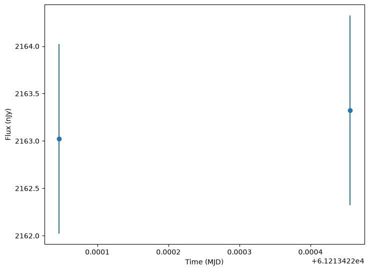
[14]:
from lightcurvelynx.utils.plotting import plot_lightcurves

lc = lightcurves["lightcurve"][0]
plot_lightcurves(
    lc["flux"],
    lc["mjd"],
    fluxerrs=lc["fluxerr"],
    filters=lc["filter"],
)
[14]:
<Axes: xlabel='Time (MJD)', ylabel='Flux (nJy)'>
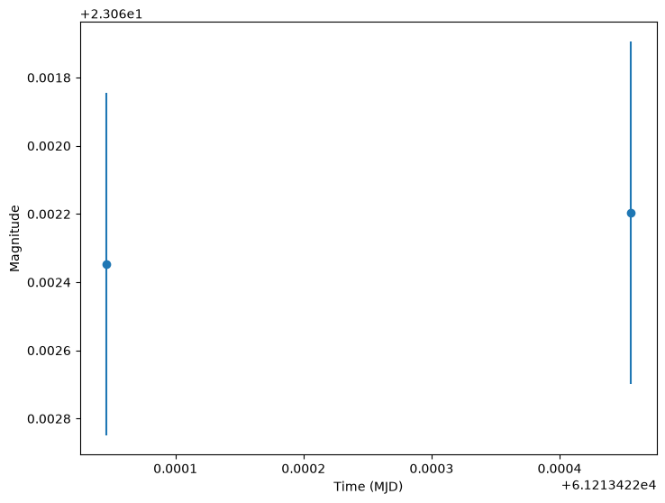
We can also plot in magnitudes (conversion is done in the function).
[15]:
plot_lightcurves(
    lc["flux"],
    lc["mjd"],
    fluxerrs=lc["fluxerr"],
    filters=lc["filter"],
    plot_magnitudes=True,
)
[15]:
<Axes: xlabel='Time (MJD)', ylabel='Magnitude'>
Reconstructing the Underlying Model
All of the information needed to reconstruct each sample’s model is included as a (flattened) dictionary in the results’ “params” column:
[16]:
print(lightcurves["params"][0])
{'NumpyRandomFunc:normal_1.loc': 9.25, 'NumpyRandomFunc:normal_1.scale': 0.05, 'NumpyRandomFunc:normal_1.function_node_result': 9.160158020481934, 'sin_wave_model.ra': 9.160158020481934, 'sin_wave_model.dec': -43.97881449496116, 'sin_wave_model.redshift': None, 'sin_wave_model.t0': 60796.0, 'sin_wave_model.distance': None, 'sin_wave_model.brightness': 2000.0, 'sin_wave_model.amplitude': 200.0, 'sin_wave_model.frequency': 0.07463545018059994, 'NumpyRandomFunc:normal_2.loc': -44.0, 'NumpyRandomFunc:normal_2.scale': 0.05, 'NumpyRandomFunc:normal_2.function_node_result': -43.97881449496116, 'NumpyRandomFunc:uniform_3.low': 0.01, 'NumpyRandomFunc:uniform_3.high': 0.1, 'NumpyRandomFunc:uniform_3.function_node_result': 0.07463545018059994}
We can convert those flattened dictionaries back to the GraphState objects (which allows us to replay the simulation) using from_dict for a single state or from_list for multiple states:
[17]:
from lightcurvelynx.graph_state import GraphState

state_0 = GraphState.from_dict(lightcurves["params"][0])
print("First sample: ", state_0)
First sample:  NumpyRandomFunc:normal_1:
    loc: 9.25
    scale: 0.05
    function_node_result: 9.160158020481934
sin_wave_model:
    ra: 9.160158020481934
    dec: -43.97881449496116
    redshift: None
    t0: 60796.0
    distance: None
    brightness: 2000.0
    amplitude: 200.0
    frequency: 0.07463545018059994
NumpyRandomFunc:normal_2:
    loc: -44.0
    scale: 0.05
    function_node_result: -43.97881449496116
NumpyRandomFunc:uniform_3:
    low: 0.01
    high: 0.1
    function_node_result: 0.07463545018059994
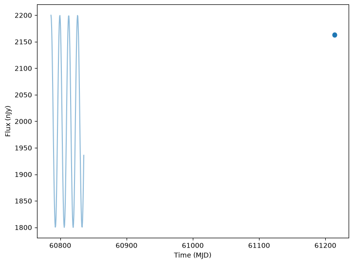
The simulation tools also have a function to generate the noise free light curves in each band over a given set of times. This returns a dictionary of filter name to band fluxes at each time. We extend the light curve out beyond the two sampled points to give a better idea of the shape.
[18]:
from lightcurvelynx.simulate import compute_single_noise_free_lightcurve

noise_free_lcs = compute_single_noise_free_lightcurve(
    model,
    state_0,
    passband_group,
    rest_frame_phase_min=-10.0,  # 10 days before t0
    rest_frame_phase_max=40.0,  # 40 days after t0
    rest_frame_phase_step=0.5,  # 2 samples per day
)
We can plot the noise free curves as a background line when plotting the light curves, using the underlying_model parameter:
[19]:
lc_0 = lightcurves["lightcurve"][0]
plot_lightcurves(
    lc_0["flux"],
    lc_0["mjd"],
    fluxerrs=lc_0["fluxerr"],
    filters=lc_0["filter"],
    underlying_model=noise_free_lcs,
)
[19]:
<Axes: xlabel='Time (MJD)', ylabel='Flux (nJy)'>
Saving Data
We can save the results of a simulation using nested-pandas to_parquet function. This will save the entire result set in a single file.
For this example, we save the results to a temporary directory.
[20]:
from pathlib import Path
import tempfile

with tempfile.TemporaryDirectory() as tmpdir:
    tmp_path = Path(tmpdir) / "simulated_lightcurves.parquet"
    lightcurves.to_parquet(tmp_path)
Since individual light curves, such as lc_0 above, are stored in pandas frames, we can save them individually using any of panda’s built-in functions.
We can also output the simulation results as a LSDB Catalog using the write_results_as_hats function. These catalogs can be read in and analyzed by the LSDB tools. Note that LSDB is not installed by default, so users will need to install it before using this function.
Conclusion
This tutorial barely scratches the surface on what LightCurveLynx can do and how it operates. The goal is to provide an overview. Interested users are encouraged to explore the other tutorial notebooks or reach out directly to the team.