Adding New Models

A major goal of LightCurveLynx is to be easily extensible so that users can create and analyze their own models. In this tutorial we look at how a user can add a custom model to simulate an astronomical phenomenon that is not already supported by LightCurveLynx.

Creating a new model node

All models are subclasses of the BasePhysicalModel class in src/lightcurvelynx/sources/physical_models.py. This class implements a bunch of helper functions to handle parameters and simulate the output of an object. Users should not subclass BasePhysicalModel directly, but rather subclass either SEDModel (which generates temporal spectral outputs) or BandfluxModel (which generates light-curve-like outputs). Depending on the model type, users only need to override a small number of functions.

For SED-type models, the user should override:

• The __init__() method sets up the parameters.

• The compute_sed() computes effect-free observations for the object in the object’s rest frame and given parameter values.

If the object has a redshift value, the SEDModel class takes care of accounting for the shift in both times and wavelengths from the observer’s frame to the rest frame (and back). So each model only needs to worry about generating fluxes in their rest frame.

For Bandflux-type models, the user should override:

• The __init__() method sets up the parameters.

• The compute_bandflux() computes effect-free observations for the object in the observer frame for a specific filter.

Effects are applied within the helper functions, so users do not need to worry about calling them from compute_sed() or compute_bandflux().

Both functions are designed to be deterministic given the parameter values (GraphState object). For models requiring random behavior, such as an AGN model using a damped random walk, a randomized seed can be included in the parameters. This allows users to produce randomized behavior on typical runs while also allowing them to reproduce previous runs to analayze behavior. For more detail on this approach, see the “Custom Models and Effects” section of the documentation.

Some models, such as those fit from observed data, may only be valid over a range of times or wavelengths. LightcurveLynx provides both the mechanisms to enforce this and to extrapolate outside those bounds. See the extrapolation notebook for more details if you need to limit the range of your model.

Parameterization

As discussed in the introduction notebook, all nodes in LightCurveLynx accept dynamic parameterization. These are parameters that change with each sampling run. For example if we have a node modeling the model’s output as a sin wave, we may want to include two parameters: the peak brightness of the object and the frequency of the underlying wave. We specify both of these parameters with the ParameterizedNode’s add_parameter() function. Behind the scenes this function does the heavy lifting to understand how the parameter is actually set during each run (from a constant, another ParameterizedNode, the computation of a function, etc.).

It is highly recommended to include the optional description argument for each parameter so users can get help on what each parameter means.

Example Model Node

Consider the example below, which implements the sin wave model. There are some details in the implementation below that we do not cover immediately (such as the get_local_params() function), but will describe below.

import numpy as np

from lightcurvelynx.models.physical_model import SEDModel


class SinModel(SEDModel):
    """A model that emits a sine wave:

    flux = brightness * sin(2 * pi * frequency * (time - t0))

    Parameters
    ----------
    brightness : `float`
        The inherent brightness
    frequency : `float`
        The frequence of the sine wave.
    **kwargs : `dict`, optional
        Any additional keyword arguments.
    """

    def __init__(self, brightness, frequency, **kwargs):
        # The call to the super's init sets up the standard physical model
        # parameters, such as ra, dec, redshift, etc.
        super().__init__(**kwargs)
        self.add_parameter(
            "brightness",
            brightness,
            description="The inherent brightness",
        )
        self.add_parameter(
            "frequency",
            frequency,
            description="The frequency of the sine wave.",
        )

    def compute_sed(self, times, wavelengths, graph_state, **kwargs):
        """Draw effect-free observations for this object.

        Parameters
        ----------
        times : `numpy.ndarray`
            A length T array of rest frame timestamps.
        wavelengths : `numpy.ndarray`, optional
            A length N array of wavelengths (in angstroms).
        graph_state : `GraphState`
            An object mapping graph parameters to their values.
        **kwargs : `dict`, optional
            Any additional keyword arguments.

        Returns
        -------
        flux_density : `numpy.ndarray`
            A length T x N matrix of SED values (in nJy).
        """
        params = self.get_local_params(graph_state)
        phases = 2.0 * np.pi * params["frequency"] * (times - params["t0"])
        single_wave = params["brightness"] * np.sin(phases)
        return np.tile(single_wave[:, np.newaxis], (1, len(wavelengths)))

/home/docs/checkouts/readthedocs.org/user_builds/lightcurvelynx/envs/latest/lib/python3.12/site-packages/tqdm/auto.py:21: TqdmWarning: IProgress not found. Please update jupyter and ipywidgets. See https://ipywidgets.readthedocs.io/en/stable/user_install.html
  from .autonotebook import tqdm as notebook_tqdm

As described above, the __init__() function adds two parameters brightness and frequency. Here they are set from the input arguments of the same name; however, as we will see below, they could be set by a variety of inputs. Each parameterized node inherits the parameters set by its parent node, and these parameters are set up in the call super().__init__(**kwargs). For the BasePhysicalModel class, these parameters include: dec, distance, ra, redshift, and t0.

We can create a model node and request information about its settable parameters.

model = SinModel(brightness=15.0, frequency=1.0, t0=0.0)
model.describe_params()

Parameters in SinModel:

ra:
    Description: The object's right ascension (in degrees)
    Source: CONSTANT with value = None

dec:
    Description: The object's declination (in degrees)
    Source: CONSTANT with value = None

redshift:
    Description: The object's redshift.
    Source: CONSTANT with value = None

t0:
    Description: The phase offset in MJD.
    Source: CONSTANT with value = 0.0

distance:
    Description: The object's luminosity distance (in pc)
    Source: CONSTANT with value = None

brightness:
    Description: The inherent brightness
    Source: CONSTANT with value = 15.0

frequency:
    Description: The frequency of the sine wave.
    Source: CONSTANT with value = 1.0

Accessing a Node’s Parameters

Each ParameterizedNode is stateless by design, so it does not store the values for any of its parameters. Instead it stores information on how to get those values when sampled. Thus the compute_sed() function must take a GraphState object that contains the parameter information. This is usually generated with a call to sample_parameters(), but will also be automatically generated internally if the evaluate_sed() function is called without this information.

The compute_sed() function can use the self.get_local_params(graph_state) to extract the current node’s parameters from the GraphState object. This function returns a dictionary mapping the parameter’s name to its value.

Evaluating the Node

The actual evaluation (computation of the SED) of the model occurs through the object’s evaluate_sed() or evaluate_bandfluxes() functions, which internally calls the compute_flux() (or compute_bandflux()) function. It is important to note that SED-type models can generate both SEDs and bandfluxes, while bandflux models can only generate bandfluxes.

Users of the node should call the evaluate_sed() or evaluate_bandfluxes() functions, since these functions perform the necessary pre- and post- computations, such as shifting the wavelengths according to the redshift (for SED-models) and applying effects (for all model types). The developer of a model only needs to implement either the compute_sed() (SED-type) or compute_bandflux() (bandflux-type) functions, though.

Note: LightCurveLynx is set up to be modular with the foundation code performing most of the heavy lifting. This includes most of the functions in SEDModel and BandfluxModel, because these base classes are set up to consistently apply transformations and effects to all their subclasses. New effects can be added by creating new subclasses of EffectModel. Thus the developers of new models should avoid overloading or modifying the evaluate_ functions unless they need to fundamentally change how effects are applied.

import matplotlib.pyplot as plt

times = np.arange(0, 4.0, 0.1)
wavelengths = np.array([100.0, 200.0])

values = model.evaluate_sed(times, wavelengths)

plt.plot(times, values[:, 0], color="blue", marker="o", linewidth=0)
plt.plot(times, 15.0 * np.sin(2.0 * np.pi * times), color="black", linewidth=1, linestyle="--", markersize=0)
plt.xlabel("Time")
plt.ylabel("Flux Density")

Text(0, 0.5, 'Flux Density')

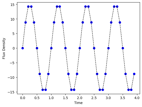
Here our new SinModel is sampling the parameters to create a GraphState object and then passing that through to compute_sed() to produce a T by W matrix where T is the number of times to sample and W is the number of wavelengths to sample.

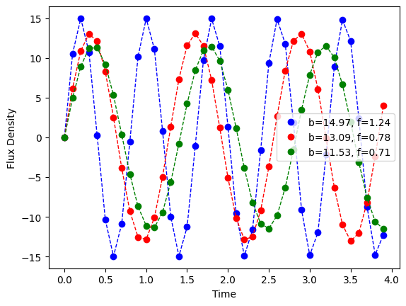
If our node’s parameters are not constant, such as brightness being generated randomly [10.0, 11.0], then we will get different results each time we evaluate the SED.

Next we use LightCurveLynx’s built-in NumpyRandomFunc node to generate the input for another node’s parameter. The underlying source is still the same SinModel class. However we have changed how we specify the parameter. Instead of assigning a constant, we assign the output of another node. In this case, the NumpyRandomFunc node wraps numpy’s random number generator and returns samples from it. As shown in the plot each of the samples comes from a sin wave with a different brightness (max value) and frequency. The legend shows the values for each curve.

from lightcurvelynx.math_nodes.np_random import NumpyRandomFunc

model = SinModel(
    brightness=NumpyRandomFunc("uniform", low=10.0, high=20.0),
    frequency=NumpyRandomFunc("uniform", low=0.5, high=1.5),
    t0=0.0,
    node_label="model",
)

# Plot three random draws from the model
for color in ["blue", "red", "green"]:
    sample = model.sample_parameters()

    # Extract the sampled parameters to use in the legend
    brightness = sample["model"]["brightness"]
    frequency = sample["model"]["frequency"]

    # Evaluate the model (using the sampled parameters) and plot the result.
    values = model.evaluate_sed(times, wavelengths, sample)
    plt.plot(
        times,
        values[:, 0],
        color=color,
        marker="o",
        linewidth=0,
        label=f"b={brightness:.2f}, f={frequency:.2f}",
    )
    plt.plot(
        times,
        brightness * np.sin(2.0 * np.pi * frequency * times),
        color=color,
        linewidth=1,
        linestyle="--",
        markersize=0,
    )
plt.legend()
plt.xlabel("Time")
plt.ylabel("Flux Density")

Text(0, 0.5, 'Flux Density')

Using Internal Functions

In the last example above, we used the NumpyRandomFunc node to generate a uniform value from [10.0, 11.0]. This provides an example of how nodes in the graph can depend on each other. But what about cases where some information in the node depends on other information provided to the node?

An example of this might be a model of an AGN where the parameterization depends on the mass of the central blackhole (blackhole_mass). We define another parameter as a function of that given parameter: accretion_rate is computed from the blackhole mass. For this second parameter, we feed information from other parameters into a function and return the result.

LightCurveLynx’s FunctionNode class provides a wrapper for such functions. The constructor takes in the function and a list of parameters. It can then be referenced directly to use its output to set parameters in other parts of the model. While the function we show below is simple (only one variable), we can use these types of function nodes to capture complex interactions. For example the BasePhysicalModel function has the ability to compute an estimated distance from a given redshift and cosmological model.

from astropy import constants

from lightcurvelynx.base_models import FunctionNode


class ToyAGN(SEDModel):
    """A toy AGN model.

    Parameters
    ----------
    blackhole_mass : float
        The black hole mass in g.
    **kwargs : `dict`, optional
        Any additional keyword arguments.
    """

    def __init__(self, blackhole_mass, **kwargs):
        super().__init__(**kwargs)

        # Add the given parameters.
        self.add_parameter("blackhole_mass", blackhole_mass, **kwargs)

        # Add the derived parameters using FunctionNodes built from the object's methods.
        # Each of these will be computed for each sample value of the input parameters.
        self.add_parameter(
            "accretion_rate",
            FunctionNode(self._compute_accretion_rate, blackhole_mass=self.blackhole_mass),
            **kwargs,
        )

    def _compute_accretion_rate(self, blackhole_mass):
        return 1.4e18 * blackhole_mass / constants.M_sun.cgs.value

    def compute_sed(self, times, wavelengths, graph_state, **kwargs):
        """Draw effect-free observations for this object.

        Parameters
        ----------
        times : `numpy.ndarray`
            A length T array of rest frame timestamps.
        wavelengths : `numpy.ndarray`, optional
            A length N array of wavelengths (in angstroms).
        graph_state : `GraphState`
            An object mapping graph parameters to their values.
        **kwargs : `dict`, optional
            Any additional keyword arguments.

        Returns
        -------
        flux_density : `numpy.ndarray`
            A length T x N matrix of SED values (in nJy).
        """
        params = self.get_local_params(graph_state)
        return np.full((len(times), len(wavelengths)), params["accretion_rate"])

To see how this works, let’s create a model where the blackhole mass is generated using a Gaussian distribution (centered on 1000x the sun’s mass with a standard deviation of 50) and look at the sampled parameters.

agn_model = ToyAGN(
    blackhole_mass=NumpyRandomFunc(
        "normal", loc=1000.0 * constants.M_sun.cgs.value, scale=50.0 * constants.M_sun.cgs.value
    ),
    node_label="toy_agn",
)

samples = agn_model.sample_parameters(num_samples=5)
print(samples)

toy_agn:
    ra: [None None None None None]
    dec: [None None None None None]
    redshift: [None None None None None]
    t0: [None None None None None]
    distance: [None None None None None]
    blackhole_mass: [1.99706504e+36 1.93014048e+36 1.91706585e+36 1.91374315e+36
 1.87748065e+36]
    accretion_rate: [1.40609393e+21 1.35897367e+21 1.34976809e+21 1.34742864e+21
 1.32189694e+21]
NumpyRandomFunc:normal_1:
    loc: [1.98840987e+36 1.98840987e+36 1.98840987e+36 1.98840987e+36
 1.98840987e+36]
    scale: [9.94204935e+34 9.94204935e+34 9.94204935e+34 9.94204935e+34
 9.94204935e+34]
    function_node_result: [1.99706504e+36 1.93014048e+36 1.91706585e+36 1.91374315e+36
 1.87748065e+36]
FunctionNode:_compute_accretion_rate_2:
    blackhole_mass: [1.99706504e+36 1.93014048e+36 1.91706585e+36 1.91374315e+36
 1.87748065e+36]
    function_node_result: [1.40609393e+21 1.35897367e+21 1.34976809e+21 1.34742864e+21
 1.32189694e+21]

What we see in the output is list of nodes, each with a corresponding list of parameters with one entry for each sample. The entries under the node=toy_agn and parameter=blackhole_mass show the five independent samples generated for the blackhole mass by the Gaussian function. Each of these serves as top level input to the model. Note that some of the parameters are None, such as the model’s RA, dec, distance, and redshift, because we did not set them.

In contrast to parameters like blackhole_mass which are generated independently from a Gaussian, other parameters are generated conditioned on existing parameters in the model. Consider the relationship between the input data and the accretion rate. From the _compute_accretion_rate() function, we can see that the accretion rate is proportional to the blackhole mass. The values of each accretion_rate sample is set deterministically from the corresponding sample of the blackhole_mass. In other words, the parameters for each sample are mathematically consistent within the sample.

Note that in addition to explicitly provided parameters we can see inherited parameters (e.g. toy_agn.ra) and internal bookkeeping parameters. An example of the latter type is the parameter function_node_result which stores a function’s computed results so it can be passed to later nodes.

More Complex Compute Functions

The heart of each model is its compute_sed() function, which determines how the node is actually simulated.

While the examples above are relatively simplistic (a sin wave or a constant output), we can made arbitrarily complicated models. We suggest that developers of new models look at the examples in src/lightcurvelynx/models/ for further demonstration.