EffectModels

In this tutorial we look at how a user can add effects to the models that we are simulating in order to make their sampled flux more realistic. Effects are transformations applied to the source’s computed flux.

LightCurveLynx supports multiple model-level effects including:

• Dust extinction (using either the extinction package or dust_extinction package.

• Microlensing (using the VBMicrolensing package)

• Multiplicative scaling (including constant dimming)

• White Noise

In addition, as shown below, users can create their own effects. You can see the Time Varying EffectModels notebook for an example of creating a more advanced custom effect model.

Applying Effects

We add effects to our models, using the BasePhysicalModel.add_effect() function, before generating samples. For example if we want to apply a basic white noise effect to a ConstantSEDModel we would use:

import numpy as np

from lightcurvelynx.effects.white_noise import WhiteNoise
from lightcurvelynx.models.basic_models import ConstantSEDModel

# Create the constant SED model.
model = ConstantSEDModel(
    brightness=10.0,
    node_label="my_constant_sed_model",
    seed=100,
)

# Create the white noise effect and add it to the model.
white_noise = WhiteNoise(white_noise_sigma=0.1)
model.add_effect(white_noise)

# Sample the flux.
state = model.sample_parameters()
times = np.array([1, 2, 3, 4, 5, 10])
wavelengths = np.array([100.0, 200.0, 300.0])
model.evaluate_sed(times, wavelengths, state)

/home/docs/checkouts/readthedocs.org/user_builds/lightcurvelynx/envs/latest/lib/python3.12/site-packages/tqdm/auto.py:21: TqdmWarning: IProgress not found. Please update jupyter and ipywidgets. See https://ipywidgets.readthedocs.io/en/stable/user_install.html
  from .autonotebook import tqdm as notebook_tqdm

array([[10.19235099,  9.87473494,  9.96950195],
       [ 9.99361306,  9.90014825, 10.10322265],
       [10.09646114, 10.16040618, 10.04793596],
       [10.02222874,  9.89056716,  9.96480422],
       [ 9.86785245, 10.00356108, 10.20290068],
       [ 9.96548982, 10.00546727,  9.94011061]])

There are a few things to note in the above code block. First, effects must be explicitly added to each model. Second, effects can contain parameters, such as the white_noise_sigma parameter above.

We can list the effects added to a model using the list_effects() function. This will return a list of all effects in the order in which they are applied.

model.list_effects()

[WhiteNoise(white_noise_sigma,white_noise_seed)]

Effect Parameters

Although effects are not a subclass of ParameterizedNode, they can include settable parameters. These parameters could be set from another parameterized node, such as a NumpyRandomFunc node or the model node itself.

An effect’s parameterized values are stored in the model node’s namespace. So the full parameter name in the previous example will be my_constant_sed_model.white_noise_sigma. Storing the effect’s parameters in the model’s namespace is done to ensure sampling consistency with the model and allow an effect to be added to multiple models without accidentally linking those models’ simulated values. For example, if we are simulating a pair of unresolved objects at significantly different redshifts (distances) we might want to apply different levels of dust extinction. Instead of creating one dust extinction effect model for each of our sources, we can create a single one and apply it to each source.

For most users, this distinction will not matter. The primary visible difference comes when manually examining the GraphState object.

Let’s we create a constant dimming effect whose strength is a random parameter sampled uniformly from [0, 1].

from lightcurvelynx.effects.basic_effects import ScaleFluxEffect
from lightcurvelynx.math_nodes.np_random import NumpyRandomFunc

# Create a new constant SED model.
model = ConstantSEDModel(
    brightness=10.0,
    node_label="my_constant_sed_model",
    seed=100,
)

# Create the constant dimming effect where its fraction is sampled.
dimming_frac = NumpyRandomFunc("uniform", low=0.0, high=1.0)
dimming_effect = ScaleFluxEffect(flux_scale=dimming_frac)

# When we add the effect, its parameters are included in the model.
model.add_effect(dimming_effect)
state = model.sample_parameters(num_samples=10)
print(state)

my_constant_sed_model:
    ra: [None None None None None None None None None None]
    dec: [None None None None None None None None None None]
    redshift: [None None None None None None None None None None]
    t0: [None None None None None None None None None None]
    distance: [None None None None None None None None None None]
    brightness: [10. 10. 10. 10. 10. 10. 10. 10. 10. 10.]
    flux_scale: [0.97168514 0.59606459 0.271116   0.52893915 0.1039099  0.65875966
 0.29506098 0.40464761 0.67551601 0.04280791]
NumpyRandomFunc:uniform_1:
    low: [0. 0. 0. 0. 0. 0. 0. 0. 0. 0.]
    high: [1. 1. 1. 1. 1. 1. 1. 1. 1. 1.]
    function_node_result: [0.97168514 0.59606459 0.271116   0.52893915 0.1039099  0.65875966
 0.29506098 0.40464761 0.67551601 0.04280791]

Note that, as expected, flux_scale is stored under my_constant_sed_model.

Each sample’s flux_scale is applied during simulation.

times = np.array([1])
wavelengths = np.array([100.0])
flux_densities = model.evaluate_sed(times, wavelengths, state)

for idx, fd in enumerate(flux_densities):
    print(f"Sample {idx}: {fd[0, 0]}")

Sample 0: 9.7168513994881
Sample 1: 5.960645910301176
Sample 2: 2.7111599935061816
Sample 3: 5.289391465959748
Sample 4: 1.0390989552993801
Sample 5: 6.587596639071628
Sample 6: 2.950609773441486
Sample 7: 4.046476060524488
Sample 8: 6.755160112026045
Sample 9: 0.4280791363874237

The ability to scale the fluxes by different multiplicative amounts enables us to use the ScaleFluxEffect to change the amplitude of pre-simulated light curves, such as LCLIB of SIMSED, or given SEDs.

Dust Maps

Dust extinction represents a more complex effect since it requires the user to specify both a dust map and an extinction function. The dust map is stored in a ParameterizedNode that uses the object’s (RA, dec) to compute ebv values. LightCurveLynx uses ExtinctionEffect which supports two different extinction packages:

• The dust_extinction package and uses the paramegter “ebv” during computation. Some extinction functions take an Rv parameter when created.

• The extinction package and uses two parameters “Av” and “Rv” during computation.

The ExtinctionEffect takes “ebv” as a settable parameter and an optional “Rv” parameter during creation. It then handles alls the necessary transformations.

Let’s look at how the ExtinctionEffect works by linking with the dust map to create a new “ebv” parameter in the model node. This “ebv” parameter is the output of the dustmap and the input to the extinction effect.

The below example requires the dust_extinction package, which is not installed by default. Users can install the pip install dust_extinction or conda install -c conda-forge dust_extinction to run this cell of the notebook.

import importlib

if importlib.util.find_spec("dust_extinction") is None:
    print("Skipping dust extinction example since dust_extinction is not installed.")
    states2 = None
else:
    from lightcurvelynx.astro_utils.dustmap import ConstantHemisphereDustMap, DustmapWrapper
    from lightcurvelynx.effects.extinction import ExtinctionEffect

    model2 = ConstantSEDModel(
        brightness=100.0,
        ra=45.0,
        dec=20.0,
        redshift=0.0,
        node_label="object",
    )

    # Create a dust map that pulls ebv values using the object's (RA, dec) values.
    dust_map = ConstantHemisphereDustMap(north_ebv=0.8, south_ebv=0.5)
    dust_map_node = DustmapWrapper(
        dust_map,
        ra=model2.ra,
        dec=model2.dec,
        node_label="dust_map",
    )

    # Create an add an extinction effect.
    ext_effect = ExtinctionEffect(
        extinction_model="CCM89",
        ebv=dust_map_node,
        frame="rest",
        r_v=3.1,
        backend="dust_extinction",
    )
    model2.add_effect(ext_effect)

    # Sample the model.
    times = np.array([1.0, 2.0, 3.0, 4.0, 5.0])
    wavelengths = np.array([7000.0, 5200.0])
    states2 = model2.sample_parameters(num_samples=3)
    model2.evaluate_sed(times, wavelengths, states2)

Skipping dust extinction example since dust_extinction is not installed.

By printing the information in the states variable, we can see a sampled ebv for each different model (RA, dec).

if states2 is not None:  # Skipped if the dust_extinction package is not installed.
    print(states2)

Alternatively, we could create an ExtinctionEffect that uses the extinction package. This package is also not installed by default. Users can install the pip install extinction to run this cell of the notebook.

import importlib

if importlib.util.find_spec("extinction") is None:
    print("Skipping extinction example since extinction is not installed.")
    states3 = None
else:
    from lightcurvelynx.astro_utils.dustmap import ConstantHemisphereDustMap, DustmapWrapper
    from lightcurvelynx.effects.extinction import ExtinctionEffect

    model3 = ConstantSEDModel(
        brightness=100.0,
        ra=45.0,
        dec=20.0,
        redshift=0.0,
        node_label="object",
    )

    # Create a dust map that pulls ebv values using the object's (RA, dec) values.
    dust_map = ConstantHemisphereDustMap(north_ebv=0.8, south_ebv=0.5)
    dust_map_node = DustmapWrapper(
        dust_map,
        ra=model3.ra,
        dec=model3.dec,
        node_label="dust_map",
    )

    # Create an add an extinction effect.
    ext_effect = ExtinctionEffect(
        extinction_model="calzetti00",
        ebv=dust_map_node,
        frame="rest",
        r_v=3.1,
        backend="extinction",
    )
    model3.add_effect(ext_effect)

    # Sample the model.
    times = np.array([1.0, 2.0, 3.0, 4.0, 5.0])
    wavelengths = np.array([7000.0, 5200.0])
    states3 = model3.sample_parameters(num_samples=3)
    model3.evaluate_sed(times, wavelengths, states3)

    print(states3)

Skipping extinction example since extinction is not installed.

Most users will want to use a more realistic dust map, such as those from the dustmaps library. For example if you had that package installed, you could create the dust map node as:

if importlib.util.find_spec("dustmaps") is not None:
    import dustmaps.sfd
    from dustmaps.config import config as dm_config

    from lightcurvelynx.astro_utils.dustmap import DustmapWrapper

    dm_config["data_dir"] = "../../data/dustmaps"
    dustmaps.sfd.fetch()
    dust_map_node = DustmapWrapper(
        dustmaps.sfd.SFDQuery(),
        ra=model2.ra,
        dec=model2.dec,
    )

Custom Effects

Users can also create their own custom effect by inheriting from the EffectModel class and overriding the apply() function.

An EffectModel object can have its own parameters (defined with a add_effect_parameter() function). Unlike a ParameterizedNode, these parameters will be added to the source object and passed to the effect as input. This means that all effect parameters will be computed during the parameter sampling phase, which keeps them consistent with the model parameters. These parameters must also be listed in the argument list for the apply() function because that is how the effect will get them.

Let’s consider the example of an effect that adds sinusoidal dimming to the flux.

from lightcurvelynx.effects.effect_model import EffectModel


class SinDimming(EffectModel):
    """A sinusoidal dimming model.

    Attributes
    ----------
    period : parameter
        The period of the sinusoidal dimming.
    """

    def __init__(self, period, **kwargs):
        super().__init__(**kwargs)
        self.add_effect_parameter("period", period)

    def apply(
        self,
        flux_density,
        times=None,
        wavelengths=None,
        period=None,
        **kwargs,
    ):
        """Apply the effect to observations (flux_density values).

        Parameters
        ----------
        flux_density : numpy.ndarray
            A length T X N matrix of flux density values (in nJy).
        times : numpy.ndarray, optional
            A length T array of times (in MJD). Not used for this effect.
        wavelengths : numpy.ndarray, optional
            A length N array of wavelengths (in angstroms). Not used for this effect.
        period : float, optional
            The period of the dimming. Raises an error if None is provided.
        **kwargs : `dict`, optional
           Any additional keyword arguments. This includes all of the
           parameters needed to apply the effect.

        Returns
        -------
        flux_density : numpy.ndarray
            A length T x N matrix of flux densities after the effect is applied (in nJy).
        """
        if period is None:
            raise ValueError("period must be provided")

        scale = 0.5 * (1.0 + np.sin(2 * np.pi * times / period))
        return flux_density * scale[:, None]

import matplotlib.pyplot as plt

model3 = ConstantSEDModel(
    brightness=100.0,
    ra=45.0,
    dec=20.0,
    redshift=0.0,
    node_label="object",
)
sin_effect = SinDimming(period=10.0)
model3.add_effect(sin_effect)

# Construct one sample of the model and its output flux.
times = np.arange(50.0)
wavelengths = np.array([7000.0, 5200.0])
fluxes = model3.evaluate_sed(times, wavelengths)

plt.plot(times, fluxes[:, 0])
plt.xlabel("Time (MJD)")
plt.ylabel("Flux Density (nJy)")

Text(0, 0.5, 'Flux Density (nJy)')

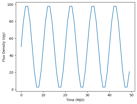
Effects can also vary their impact depending on both time and wavelength. For more complex examples see the time_varying_effects.ipynb notebook.

Random Effects

LightCurveLynx supports a combination of random effects, such as the WhiteNoise effect with the ability to deterministically reproduce models given the GraphState object. It does this by creating a random seed for the effect, such as the white_noise_seed parameter and using that to control the randomness of the effect. If a seed is manually specified during a run (as when replaying a previous run) the known seed will produce deterministic results. Otherwise the randomly choose seed will produce random results.