Sampling Parameters

In this tutorial we explore the mechanisms for sampling the parameters used to simulate physical objects.

Time domain models are often defined by numerous parameters for everything from position on the sky (RA, Dec) to inherent physical quantities (hostmass) to purely functional parameters (curve decay rate). You can think of these parameters as the variables in the mathematical equations. For realistic models these parameters are not independent. Parameters may be sampled based on the values of other (hyper)parameters or computed directly from other parameters. For example an SN Ia model may use an X1 parameter which is computed from the hostmass and a C parameter which is sampled based on hyperparameters.

LightCurveLynx provides a flexible framework for defining these relationships and sampling the parameters. At the heart of this sampling are nodes (or ParameterizedNode objects), which represent computational units for working with parameters. Each node defines a recipe for computing its internal parameters. Some nodes are simple computations for a single parameter, such as drawing from a Gaussian distribution or performing a computation of X1 from hostmass. Other nodes contain a series of related internal parameters that are used together. For example models (BasePhysicalModel objects) are themselves nodes with all the parameters for the object they represent.

Below is the example of a simple SN Ia model. The nodes are shown in light blue, the fixed parameters as grey circles, and the sampled parameters as white circles. The blue arrows represent the dependencies between parameters.

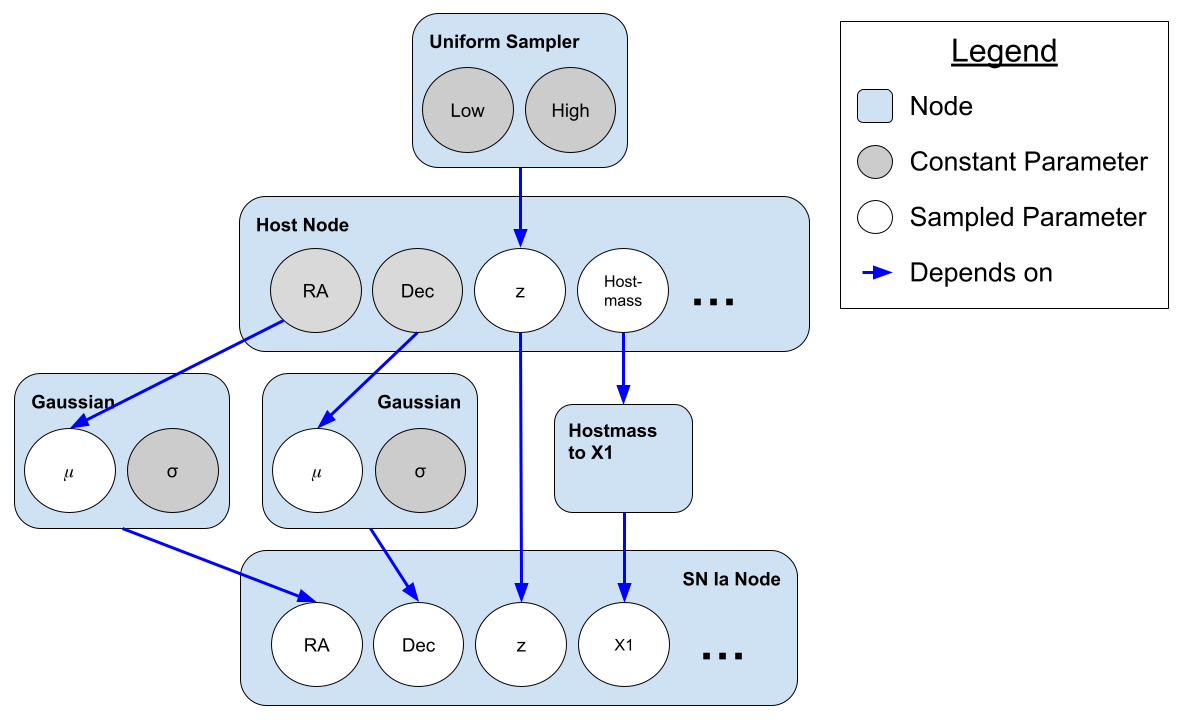
From an astronomical point of view, the model contains two objects: a host and a SN Ia. These nodes have parameters indicating position, redshift, and so forth. For this simulation graph, the position of the host is fixed but the position of the SN Ia is sampled based on Gaussian perturbations of the host’s position. Redshift (z) works the opposite way. The host’s redshift is sampled from a uniform distribution (defined by two fixed hyperparameters) and the SN Ia’s redshift is copied directly from that of its host.

Parameter dependencies are set via the arguments of a ParameterizedNode or its subclass as we will see below.

The combined values of all the parameters in the graph define a single sample of the model’s parameters.

GraphState

The ParameterizedNode objects are stateless and do not store any information about the values of the parameters. Instead, all information about a given simulation’s parameterization is stored in a GraphState object. These saved values include not only the settings of the physical object being simulated, such as its redshift, but also parameters of prior distributions and internal bookkeeping values. Most users will not need to interact directly with the GraphState object, but we provide a quick overview here for completeness.

Users can think of the GraphState as a nested dictionary where parameters are indexed by two levels. In the first level, the node label tells the code which object the parameter belongs to. This level of identification is necessary to allow different stages to use parameters with the same name. For example, in the graph above we can see that both the host and the supernova have RA values that might be very slightly different. If we are blending many objects, we could have many different RA values. In the second level of the GraphState, the parameter name maps to the actual sampled values.

As a concrete example, let’s look at a static object with a parameter for brightness. We use the sample_parameters() function to generate a GraphState.

import numpy as np

from lightcurvelynx.models.basic_models import ConstantSEDModel

source = ConstantSEDModel(brightness=10.0, node_label="my_static_source")
state = source.sample_parameters()
print(state)

/home/docs/checkouts/readthedocs.org/user_builds/lightcurvelynx/envs/latest/lib/python3.12/site-packages/tqdm/auto.py:21: TqdmWarning: IProgress not found. Please update jupyter and ipywidgets. See https://ipywidgets.readthedocs.io/en/stable/user_install.html
  from .autonotebook import tqdm as notebook_tqdm

my_static_source:
    ra: None
    dec: None
    redshift: None
    t0: None
    distance: None
    brightness: 10.0

You can see the GraphState object contains an entry for our single node (“my_static_source”) with subentries for all the parameters. Even though we only set a single parameter (brightness), the ConstantSEDModel object contains a series of other parameters that are inherited from the PhysicalModel base class such as RA, Dec, and redshift. Parameters that are not set use a given default value (in this case None).

It is important to note that the ConstantSEDModel object itself is stateless. In fact all ParameterizedNode objects are stateless. We do not store any of the parameter information internally. The nodes themselves are just recipes for operating on the GraphState object. This decoupling of state from the model objects ensures internal consistency between the parameters and allows for distributed computation.

Multiple Samples

Generating a single sample at a time adds significant overhead. If we want to generate 10,000 light curves from 10,000 Type Ia supernovae, we do not want to have to call the sampling function 10,000 separate times in a loop. For this reason, LightCurveLynx supports the vectorized generation of parameters and the GraphState objects also support the storage of multiple samples with a third layer of nesting.

state = source.sample_parameters(num_samples=5)
print(state)

my_static_source:
    ra: [None None None None None]
    dec: [None None None None None]
    redshift: [None None None None None]
    t0: [None None None None None]
    distance: [None None None None None]
    brightness: [10. 10. 10. 10. 10.]

where each (node name, parameter name) pair now maps to an array of samples. Individual values for a single sample and parameter can be accessed with array notation:

state["my_static_source"]["brightness"][2]

np.float64(10.0)

The i-th entries of each parameter represent a single sampling of parameter space and are mutually consistent. For example the position of the i-th object would be given by the tuple (state[“my_static_source”][“ra”][i], state[“my_static_source”][“dec”][i]).

Note: Care must be taken when writing code that directly accesses the GraphState object as it will return scalars when it stores a single value and arrays otherwise.

We can extract a single sample of all parameters with the extract_single_sample() function.

print(state.extract_single_sample(2))

my_static_source:
    ra: None
    dec: None
    redshift: None
    t0: None
    distance: None
    brightness: 10.0

This accessor allows us to take the parameters for multiple simulated objects and extract those to create a single one of the objects.

Alternate Accessors

You can also use a ParameterizedNode object to extract its own parameters without knowing the node’s name. This is particularly useful for computations within the object. The function get_local_params() return a dictionary of all parameters for this node. And the function get_param() looks up the value of a single parameter. Both functions take a GraphState object.

nodes_params = source.get_local_params(state)
print(nodes_params)

brightness = source.get_param(state, "brightness")
print(f"brightness = {brightness}")

{'ra': array([None, None, None, None, None], dtype=object), 'dec': array([None, None, None, None, None], dtype=object), 'redshift': array([None, None, None, None, None], dtype=object), 't0': array([None, None, None, None, None], dtype=object), 'distance': array([None, None, None, None, None], dtype=object), 'brightness': array([10., 10., 10., 10., 10.])}
brightness = [10. 10. 10. 10. 10.]

Parameterized Nodes

As described above, all parameters are generated and used by ParameterizedNode objects. The ParameterizedNode base class wraps the complexity of how parameters are linked together, how they are sampled, and how the GraphState is updated, so that users only need to define the computations themselves.

The ConstantSEDModel object we used above is a simple example of a ParameterizedNode; it takes input parameters and operates on them to generate flux from a brightness parameter. All LightCurveLynx models are subclasses of PhysicalModel which is itself a subclass of ParameterizedNode.

Other ParameterizedNode classes can be used to generate parameters from a given distribution or compute a new parameter from a combination of input parameters. Consider the NumpyRandomFunc class which wraps numpy’s random number generators. This class takes the name of the distribution and input parameters specific to that distribution. It outputs a parameter (by default called “function_node_result”) from that distribution.

from lightcurvelynx.math_nodes.np_random import NumpyRandomFunc

brightness_func = NumpyRandomFunc("uniform", low=11.0, high=15.5)
state = brightness_func.sample_parameters(num_samples=10)
print(state)

NumpyRandomFunc:uniform_0:
    low: [11. 11. 11. 11. 11. 11. 11. 11. 11. 11.]
    high: [15.5 15.5 15.5 15.5 15.5 15.5 15.5 15.5 15.5 15.5]
    function_node_result: [12.48938801 13.11395497 15.30248539 14.34140969 11.40430155 14.53923846
 11.81166575 11.64542357 11.12649959 13.84869601]

Here we can see that “low” and “high” are stored in the GraphState as input parameters along with the sampled values (which are saved as “function_node_result”).

We can access the list of all parameters within a specific node:

print(brightness_func.list_params())

['low', 'high', 'function_node_result']

or display a detailed breakdown of their details

brightness_func.describe_params()

Parameters in NumpyRandomFunc:uniform_0:

low:
    Description: Input argument for function.
    Source: CONSTANT with value = 11.0

high:
    Description: Input argument for function.
    Source: CONSTANT with value = 15.5

function_node_result:
    Description: Output result of function.
    Source: Result of computation within this node

Chaining Nodes

To be useful, we need to be able to feed the output parameter of one node into the input parameter of another node. This allows us to create a statistical graph of parameters.

For example we could create a ConstantSEDModel node where the brightness is sampled from the a Gaussian distribution. For nodes that produce a single output value (like our NumpyRandomFunc node), we can do this directly by using the node object in the arguments. This links the output of that node to the given input parameter.

brightness_dist = NumpyRandomFunc("normal", loc=20.0, scale=2.0, node_label="brightness_dist")
source = ConstantSEDModel(brightness=brightness_dist, node_label="test_source")
state = source.sample_parameters(num_samples=10)
print(state)

test_source:
    ra: [None None None None None None None None None None]
    dec: [None None None None None None None None None None]
    redshift: [None None None None None None None None None None]
    t0: [None None None None None None None None None None]
    distance: [None None None None None None None None None None]
    brightness: [19.46591265 17.83641397 18.07938993 19.11397799 18.59452428 19.70519575
 21.92752989 19.03015675 19.26070792 18.77798967]
brightness_dist:
    loc: [20. 20. 20. 20. 20. 20. 20. 20. 20. 20.]
    scale: [2. 2. 2. 2. 2. 2. 2. 2. 2. 2.]
    function_node_result: [19.46591265 17.83641397 18.07938993 19.11397799 18.59452428 19.70519575
 21.92752989 19.03015675 19.26070792 18.77798967]

Note that when we print out the GraphState now, it includes information for both the NumpyRandomFunc and ConstantSEDModel nodes. It is effectively capturing the full state of the system.

Each instance of the object’s brightness is sampled from a Gaussian distribution with the corresponding “loc” and “scale” parameters. This is an important distinction from how we might normally think of input arguments in Python. ConstantSEDModel is not getting a single value of “brightness” in its constructor, but rather is being told where to get a new value of “brightness” for each sampling run.

We can demonstrate the importance of consistency by adding a third level of chaining. We generate the Gaussian’s mean from a prior distribution.

brightness_mean = NumpyRandomFunc("uniform", low=20.0, high=30.0, node_label="brightness_mean")
brightness_dist = NumpyRandomFunc("normal", loc=brightness_mean, scale=2.0, node_label="gauss")
source = ConstantSEDModel(brightness=brightness_dist, node_label="test")
state = source.sample_parameters(num_samples=10)
print(state)

test:
    ra: [None None None None None None None None None None]
    dec: [None None None None None None None None None None]
    redshift: [None None None None None None None None None None]
    t0: [None None None None None None None None None None]
    distance: [None None None None None None None None None None]
    brightness: [28.46495094 24.02035193 29.9148437  24.27948066 25.91856008 34.40484558
 19.63685999 23.24975666 25.26152129 19.86461243]
brightness_mean:
    low: [20. 20. 20. 20. 20. 20. 20. 20. 20. 20.]
    high: [30. 30. 30. 30. 30. 30. 30. 30. 30. 30.]
    function_node_result: [29.85589467 24.3646837  29.00082237 23.19855226 27.16496914 29.09384067
 21.04230473 26.68159048 23.70208701 22.17882616]
gauss:
    loc: [29.85589467 24.3646837  29.00082237 23.19855226 27.16496914 29.09384067
 21.04230473 26.68159048 23.70208701 22.17882616]
    scale: [2. 2. 2. 2. 2. 2. 2. 2. 2. 2.]
    function_node_result: [28.46495094 24.02035193 29.9148437  24.27948066 25.91856008 34.40484558
 19.63685999 23.24975666 25.26152129 19.86461243]

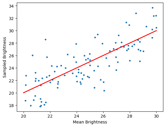
Now during each sampling instance we first generate a mean for our Gaussian distribution and then generate a brightness given that mean parameter.

import matplotlib.pyplot as plt

state = source.sample_parameters(num_samples=100)

mean_vals = state["gauss"]["loc"]
brightness_vals = state["test"]["brightness"]
plt.plot(mean_vals, brightness_vals, marker=".", linewidth=0)
plt.plot([20.0, 30.0], [20.0, 30.0], linewidth=2, color="red")
plt.xlabel("Mean Brightness")
plt.ylabel("Sampled Brightness")

Text(0, 0.5, 'Sampled Brightness')

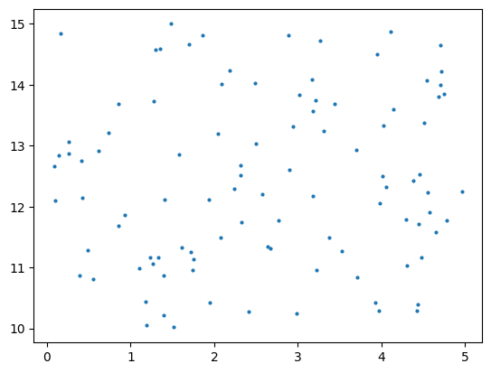
NumpyRandomFunc node can also be used to draw from multivariate distributions where each sample is a vector of values. In the following example each sample consists of a two dimensional point with the x value drawn uniformly (0.0, 10) and the y value drawn uniformly (5.0, 15.0). Note that in this case each entry for example sample is generated independently (see the NumpyMultivariateNormalFunc for correlated output).

low = [0.0, 10.0]
high = [5.0, 15.0]
np_node = NumpyRandomFunc("uniform", low=low, high=high, node_label="xy", size=2)

# Sample the multivariate normal distribution
graph_state = np_node.sample_parameters(num_samples=100)
x = graph_state["xy"]["function_node_result"][:, 0]
y = graph_state["xy"]["function_node_result"][:, 1]
_ = plt.scatter(x, y, marker=".", linewidth=0)

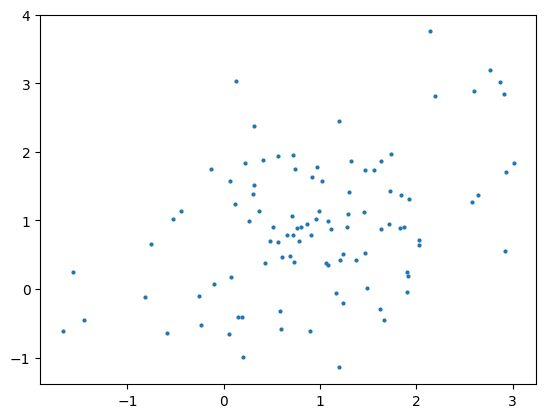
There are a few functions that are unsupported by the NumpyRandomFunc node as vectorized sampling requires a slightly different format. We provide alternative implementations:

• The “choice” sampling is implemented by the GivenValueSampler node.

• The “multivariate_normal” sampling is implemented by the NumpyMultivariateNormalFunc node.

from lightcurvelynx.math_nodes.np_random import NumpyMultivariateNormalFunc

mean = [1.0, 1.0]
cov = [[1.0, 0.5], [0.5, 1.0]]
np_node = NumpyMultivariateNormalFunc(mean=mean, cov=cov, node_label="xy")

# Sample the multivariate normal distribution
graph_state = np_node.sample_parameters(num_samples=100)
x = graph_state["xy"]["function_node_result"][:, 0]
y = graph_state["xy"]["function_node_result"][:, 1]
_ = plt.scatter(x, y, marker=".", linewidth=0)

Function Nodes

Sampling functions, such as those provided by numpy, are only one type of function that we might want to use to generate parameters. We might want to sample from other functions or apply a mathematical transform to multiple input parameters to compute a new parameter. LightCurveLynx contains numerous built-in classes to support these types of computations as well as the ability to define custom FunctionNode objects.

Creating New Function Nodes

Importantly, you can use a FunctionNode that takes input parameter(s) and produces output parameter(s) during the generation. FunctionNode is a subclass of ParameterizedNode that wraps the functionality of collecting the inputs, running the computations, and storing the output. For a tutorial of creating custom nodes see the Creating Custom Function Nodes notebook.

Basic Math Nodes

It would be tiresome to manually generate a FunctionNode object or class for every small mathematical function we need to use. As such LightCurveLynx also provides the BasicMathNode, which will take a string and (safely) compile the mathematical expression into a function. It can support most of the basic math functions that are common to the math, numpy, and jax.numpy libraries, including addition, subtraction, multiplication, division, logarithms, exponents/powers, degree/radian conversions, trig functions, absolute value, ceiling, and floor.

from lightcurvelynx.math_nodes.basic_math_node import BasicMathNode

math_node = BasicMathNode("a + b", a=5.0, b=10.0)
print(math_node.sample_parameters(num_samples=1))

math_node2 = BasicMathNode("cos(radians(a)) * abs(b) - c", a=45.0, b=-10.0, c=1.0)
print(math_node2.sample_parameters(num_samples=1))

BasicMathNode:eval_0:
    a: 5.0
    b: 10.0
    function_node_result: 15.0
BasicMathNode:eval_0:
    a: 45.0
    b: -10.0
    c: 1.0
    function_node_result: 6.0710678118654755

A full list of supported functions can be found with the list_functions() function.

BasicMathNode.list_functions()

['abs',
 'acos',
 'acosh',
 'asin',
 'asinh',
 'atan',
 'atan2',
 'cos',
 'cosh',
 'ceil',
 'degrees',
 'deg2rad',
 'e',
 'exp',
 'fabs',
 'floor',
 'log',
 'log10',
 'log2',
 'max',
 'min',
 'pi',
 'pow',
 'power',
 'radians',
 'rad2deg',
 'sin',
 'sinh',
 'sqrt',
 'tan',
 'tanh',
 'trunc']

Nodes with Multiple Computed Values

Some nodes might produce multiple computed values. A simple example of this is sampling positions from the footprint of a survey. You cannot sample RA and dec independently. Instead you need to generate a pair of values that works with the survey.

from lightcurvelynx.math_nodes.ra_dec_sampler import UniformRADEC

uniform_sampler = UniformRADEC(node_label="uniform")
print(uniform_sampler.sample_parameters(num_samples=1))

uniform:
    ra: 256.34957676524016
    dec: -12.59914012040053

Each of the outputs is saved as its own parameter for this node. The values are computed during sampling and stored in the GraphState entry for the function node. As we will see in the next section, we then use the dot notation to feed these computed values into other nodes. For more detail see the Creating Custom Function Nodes notebook.

Linked (Copied) Parameters

Often the values of one node might depend on the values of another that are not the result of a function. A great case of this is a source/host pair where the location of the source depends on that of the host. We can access another node’s sampled parameters using a . notation: {model_object}.{parameter_name}

ra_node = NumpyRandomFunc("uniform", low=0.0, high=360.0)
host = ConstantSEDModel(brightness=15.0, ra=ra_node, dec=2.0, node_label="host")
source = ConstantSEDModel(brightness=10.0, ra=host.ra, dec=host.dec, node_label="source")
state = source.sample_parameters(num_samples=100)

plt.plot(state["host"]["ra"], state["source"]["ra"], marker="o", linewidth=0)
plt.plot([0.0, 360.0], [0.0, 360.0], linewidth=1, alpha=0.5, color="red")
plt.xlabel("Host RA")
plt.ylabel("Source RA")

Text(0, 0.5, 'Source RA')

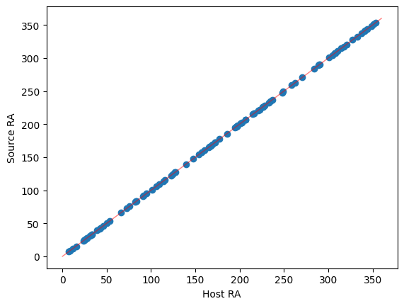
Again it is important to remember that the ParameterizedNodes are stateless and these parameters are not values stored in the Python objects themselves. In the creation of the source object, we are not setting its ra argument to the value stored in host.ra. Rather we are providing the new source node with instructions that, during each sample, it should copy the corresponding value from the host node’s ra value.

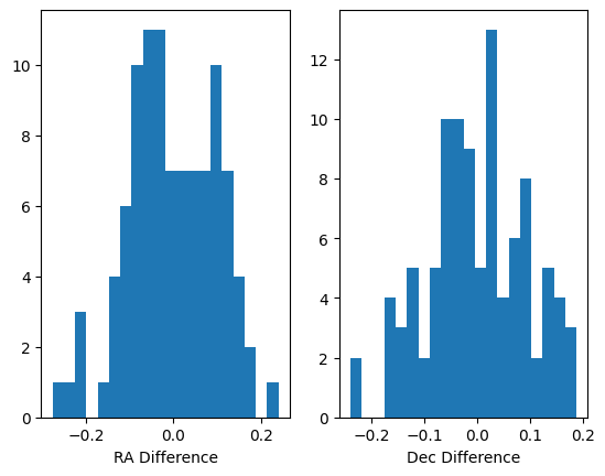
This means that we can combine the node-parameter references with functional nodes to perform actions such as sampling with noise.

Here we generate the host’s (RA, Dec) from a uniform patch of the sky and then generate the object’s (RA, Dec) using a Gaussian distribution centered on the host’s position. For each sample the host and source should be close, but not necessarily identical.

host = ConstantSEDModel(
    brightness=15.0,
    ra=NumpyRandomFunc("uniform", low=10.0, high=150.0),
    dec=NumpyRandomFunc("uniform", low=-10.0, high=10.0),
    node_label="host",
)

source = ConstantSEDModel(
    brightness=100.0,
    ra=NumpyRandomFunc("normal", loc=host.ra, scale=0.1),
    dec=NumpyRandomFunc("normal", loc=host.dec, scale=0.1),
    node_label="source",
)
state = source.sample_parameters(num_samples=100)

ra_diffs = state["source"]["ra"] - state["host"]["ra"]
dec_diffs = state["source"]["dec"] - state["host"]["dec"]

ax = plt.figure().subplots(1, 2)
ax[0].hist(ra_diffs, bins=20)
ax[0].set_xlabel("RA Difference")

ax[1].hist(dec_diffs, bins=20)
ax[1].set_xlabel("Dec Difference")

Text(0.5, 0, 'Dec Difference')

Again we can access all the information for a single sample. Here we see the full state tracked by the system. In addition to the host and source nodes we created, the information for the functional nodes is tracked.

single_sample = state.extract_single_sample(0)
print(str(single_sample))

NumpyRandomFunc:uniform_3:
    low: 10.0
    high: 150.0
    function_node_result: 12.70244367872686
host:
    ra: 12.70244367872686
    dec: 7.2193719916346915
    redshift: None
    t0: None
    distance: None
    brightness: 15.0
NumpyRandomFunc:uniform_4:
    low: -10.0
    high: 10.0
    function_node_result: 7.2193719916346915
NumpyRandomFunc:normal_1:
    loc: 12.70244367872686
    scale: 0.1
    function_node_result: 12.703263285570896
source:
    ra: 12.703263285570896
    dec: 7.345044694822772
    redshift: None
    t0: None
    distance: None
    brightness: 100.0
NumpyRandomFunc:normal_5:
    loc: 7.2193719916346915
    scale: 0.1
    function_node_result: 7.345044694822772

It is interesting to note that functional nodes themselves are parameterized nodes, allowing for more complex forms of chaining. For example we could set the low parameter from one of the NumpyRandomFuncs from another function node. This allows us to specify priors and complex distributions.

Similarly we can now make the input parameters of one node depend on a function of parameters from other nodes. We can arbitrarily chain the computations.

# Create a host galaxy with a random brightness.
host = ConstantSEDModel(
    brightness=NumpyRandomFunc("uniform", low=1.0, high=5.0),
    node_label="host",
)

# Create the brightness of the source as a uniformly sampled foreground brightness
# added to the 80% of the host's brightness (background).
source_brightness = BasicMathNode(
    "0.8 * val1 + val2",
    val1=host.brightness,
    val2=NumpyRandomFunc("uniform", low=1.0, high=2.0),
    node_label="plus_80percent",
)

source = ConstantSEDModel(
    brightness=source_brightness,
    node_label="source",
)
state = source.sample_parameters(num_samples=10)
print(f"Host Brightness: {state['host']['brightness']}")
print(f"Source Brightness: {state['source']['brightness']}")

Host Brightness: [3.28781862 1.03623508 1.22964727 4.85180844 1.23933791 1.70989989
 2.2462267  2.65542273 1.47452901 1.59220768]
Source Brightness: [3.88419024 2.56001008 2.72748639 4.94540598 2.88412629 3.02868652
 3.61094275 3.40179491 2.95727475 2.90124453]

While we use a BasicMathNode to compute the combined brightness to illustrate chaining above, we would often prefer to use a AdditiveMultiObjectModel to represent a combination of fluxes.

Conclusion

LightCurveLynx provides significant flexibility in how parameters can be defined, allowing a users to create complex statistical models. The specification is meant to be familiar to users of Python by using direct assignment (argument=object) for functions and the . notation (argument=object.parameter) for references parameters. Internally LightCurveLynx manages the various references so that each new sample regenerates the instances of the all the parameters in the model in a statistically consistent way.

This tutorial only provides an introduction to the full sampling system, which can support additional operations including:

• Multi-output functions

• Efficient vectorized computations for large numbers of samples

• Seeding of random number generation and isolation of subgraphs for testing

These concepts (and others) will be demonstrated in future tutorials and in the code.