Building Simple Models

In this tutorial we look at how to build a simple model and sample the parameters from a variety of basic sources. For more complex sampling see the notebooks: sampling.ipynb, adding_models.ipynb, and using_pzflow.ipynb.

Parameterized Nodes

All sources of information in LightCurveLynx live as ParameterizedNode objects. This allows us to link the nodes (and their variables) together and sample them as a single block. As you will see in this tutorial, most of the nodes are specific to the object that you want to simulate. For example if we wanted to create a model with constant brightness in the night sky with a brightness of 10, we could use:

import matplotlib.pyplot as plt
import numpy as np

from lightcurvelynx.models.basic_models import ConstantSEDModel

model = ConstantSEDModel(brightness=10.0, node_label="a_star")

/home/docs/checkouts/readthedocs.org/user_builds/lightcurvelynx/envs/stable/lib/python3.12/site-packages/tqdm/auto.py:21: TqdmWarning: IProgress not found. Please update jupyter and ipywidgets. See https://ipywidgets.readthedocs.io/en/stable/user_install.html
  from .autonotebook import tqdm as notebook_tqdm

Users can get information about the parameterized node using Python’s builtin help() function or display a list of the parameters with the describe_params() function.

model.describe_params()

Parameters in a_star:

ra:
    Description: The object's right ascension (in degrees)
    Source: CONSTANT with value = None

dec:
    Description: The object's declination (in degrees)
    Source: CONSTANT with value = None

redshift:
    Description: The object's redshift.
    Source: CONSTANT with value = None

t0:
    Description: The phase offset in MJD.
    Source: CONSTANT with value = None

distance:
    Description: The object's luminosity distance (in pc)
    Source: CONSTANT with value = None

brightness:
    Description: The inherent brightness of the object.
    Source: CONSTANT with value = 10.0

A ParameterizedNode can then be sampled with the sample_parameters() function. This samples the internal parameters of the model. For example we might be sampling an object’s brightness (as with the constant SED model), a host galaxy’s mass, or even the (RA, dec) position of the observations. The sample_parameters() function returns a special data structure, the GraphState, that captures this state and can later be fed into the models to generate fluxes.

Note: Users do not need to know the details of the GraphState storage, only that it can be accessed like a dictionary using the node’s label and the variable name.

state = model.sample_parameters(num_samples=10)
state["a_star"]["brightness"]

array([10., 10., 10., 10., 10., 10., 10., 10., 10., 10.])

The sample function produced 10 independent samples of our system’s state.

The brightness values of these samples are not particularly interesting because we were sampling from a fixed parameter. The brightness is always 10.0. However LightCurveLynx allows the user to set a node’s parameter from a variety of sources including constants (as with 10.0 above), the values stored in other nodes, or even the results of a “functional” or “computation” type node (more about that later).

LightCurveLynx includes the built-in NumpyRandomFunc which will sample from a given numpy function and use the results to set a given parameter.

from lightcurvelynx.math_nodes.np_random import NumpyRandomFunc

brightness_func = NumpyRandomFunc("uniform", low=11.0, high=15.5)
model2 = ConstantSEDModel(brightness=brightness_func, node_label="a_star_2")
state = model2.sample_parameters(num_samples=10)

state["a_star_2"]["brightness"]

array([12.75165308, 12.32174466, 12.91301524, 14.06416608, 12.67579947,
       11.00144668, 13.55692642, 14.92296906, 12.28495187, 12.13985863])

Now each of our 10 samples use different a different brightness value.

We can make the distributions of objects more interesting by using combinations of randomly generated parameters. Different random generators can be specified for different parameters such as brightness and redshift. For example we can sample the brightness from a Gaussian distribution and sample the redshift from a uniform distribution.

model3 = ConstantSEDModel(
    brightness=NumpyRandomFunc("normal", loc=20.0, scale=2.0),
    redshift=NumpyRandomFunc("uniform", low=0.1, high=0.5),
    node_label="test",
)

num_samples = 10
state = model3.sample_parameters(num_samples=num_samples)
for i in range(num_samples):
    print(f"{i}: brightness={state['test']['brightness'][i]} redshift={state['test']['redshift'][i]}")

0: brightness=19.531825276477004 redshift=0.2873696772105765
1: brightness=21.775325842320395 redshift=0.4580616306472578
2: brightness=16.238710239700932 redshift=0.3427928604581785
3: brightness=14.98381301724366 redshift=0.3528576366343774
4: brightness=19.24499874700299 redshift=0.2778313431835847
5: brightness=22.64911422618441 redshift=0.11588533700549704
6: brightness=15.972127065068278 redshift=0.3065054510165386
7: brightness=23.717914986566154 redshift=0.473148996677457
8: brightness=19.135059194848107 redshift=0.22526768978359435
9: brightness=19.386913675215645 redshift=0.23682628999470523

The sampling process creates vectors of samples for each parameter such that the i-th value of each parameter is from the same sampling run. So in the output above, sample 0 consists of all the parameter values for that sample (everything at index=0), sample 1 consists of all parameter values for that sample (everything at index=1), and so forth. This is critically important once we start dealing with parameters that are not independent. We might want to choose the host galaxy’s mass and redshift from a joint distribution. Alternatively, as we will see below, we will often want to compute one parameter as a mathematical transform of another or sample one parameter based on the value of another. In all of these cases it is important that we can access the parameters that were generated together and that these parameters stay consistent.

We can slice out a single sample using extract_single_sample() and display it.

single_sample = state.extract_single_sample(0)
print(str(single_sample))

test:
    ra: None
    dec: None
    redshift: 0.2873696772105765
    t0: None
    distance: None
    brightness: 19.531825276477004
NumpyRandomFunc:uniform_1:
    low: 0.1
    high: 0.5
    function_node_result: 0.2873696772105765
NumpyRandomFunc:normal_2:
    loc: 20.0
    scale: 2.0
    function_node_result: 19.531825276477004

You’ll notice that there are more parameters than we manually set. Some of these are for internal bookkeeping. Parameters are created automatically by the nodes if needed. In general the user should not need to worry about these extra parameters. They can access the ones of interest with the dictionary notation.

Function Nodes

Sampling functions, such as those provided by numpy, are only one type of function that we might want to use to generate parameters. We might want to sample from other functions or apply a mathematical transform to multiple input parameters to compute a new parameter. For example consider the case of computing the distmod parameter from redshift. We can do this using the information about the cosmology, such as provided by astropy’s FlatLambdaCDM class:

from astropy.cosmology import FlatLambdaCDM

cosmo_obj = FlatLambdaCDM(H0=73.0, Om0=0.3)
redshifts = np.array([0.1, 0.2, 0.3])
distmods = cosmo_obj.distmod(redshifts).value
print(distmods)

[38.22408047 39.8651567  40.86433594]

Importantly, you can use a FunctionNode that takes input parameter(s) and produces output parameter(s) during the generation. FunctionNode is a subclass of ParameterizedNode that wraps the functionality of collecting the inputs, running the computations, and storing the output. The user simply needs to provide the function node with the function it will use and the parameters. For example, LightCurveLynx has a DistModFromRedshift class that wraps the previous operation.

The below code samples a redshift uniformly from [0.1, 0.5], uses it to compute the distmod parameter, and sets that.

from lightcurvelynx.astro_utils.snia_utils import DistModFromRedshift

distmod_obj = DistModFromRedshift(
    H0=73.0, Omega_m=0.3, redshift=NumpyRandomFunc("uniform", low=0.1, high=0.5)
)

or more concretely, we can create our own FunctionNode that computes y = m * x + b.

from lightcurvelynx.base_models import FunctionNode


def _linear_eq(x, m, b):
    """Compute y = m * x + b"""
    return m * x + b


func_node = FunctionNode(
    _linear_eq,  # First parameter is the function to call.
    x=NumpyRandomFunc("uniform", low=0.0, high=10.0),
    m=5.0,
    b=-2.0,
)
print(func_node.sample_parameters(num_samples=1))

NumpyRandomFunc:uniform_1:
    low: 0.0
    high: 10.0
    function_node_result: 9.820984776654665
FunctionNode:_linear_eq_0:
    x: 9.820984776654665
    m: 5.0
    b: -2.0
    function_node_result: 47.10492388327333

The first parameter of the function node is the input function, such as our linear equation above. Each input into the function must be included as a named parameter, such as x, m, and b above. If any of the input parameters are missing the code will give an error.

Here we use constants for m and b so we use the same linear formulation for each sample. Only the value of x changes. However we could have also used function nodes, including sampling functions, to set m and b. In that case it is important to remember that each of our results sample will be the result of a sampling of all the variable parameters.

It would be tiresome to manually generate a FunctionNode object or class for every small mathematical function we need to use. As such LightCurveLynx also provides the BasicMathNode, which will take a string and (safely) compile the mathematical expression into a function.

from lightcurvelynx.math_nodes.basic_math_node import BasicMathNode

math_node = BasicMathNode("a + b", a=5.0, b=10.0)
print(math_node.sample_parameters(num_samples=1))

BasicMathNode:eval_0:
    a: 5.0
    b: 10.0
    function_node_result: 15.0

Linked Parameters / Nodes

Often the values of one node might depend on the values of another. A great case of this is a source/host pair where the location of the object depends on that of the host. We can access another node’s sampled parameters using a . notation: {model_object}.{parameter_name}

host = ConstantSEDModel(brightness=15.0, ra=1.0, dec=2.0, node_label="host")
source = ConstantSEDModel(brightness=10.0, ra=host.ra, dec=host.dec, node_label="source")
state = source.sample_parameters(num_samples=5)

for i in range(5):
    print(
        f"{i}: Host=({state['host']['ra'][i]}, {state['host']['dec'][i]})"
        f"Source=({state['source']['ra'][i]}, {state['source']['dec'][i]})"
    )

0: Host=(1.0, 2.0)Source=(1.0, 2.0)
1: Host=(1.0, 2.0)Source=(1.0, 2.0)
2: Host=(1.0, 2.0)Source=(1.0, 2.0)
3: Host=(1.0, 2.0)Source=(1.0, 2.0)
4: Host=(1.0, 2.0)Source=(1.0, 2.0)

We can combine the node-parameter references with functional nodes to perform actions such as sampling with noise.

Here we generate the host’s (RA, dec) from a uniform patch of the sky and then generate the source’s (RA, dec) using a Gaussian distribution centered on the host’s position. For each sample the host and source should be close, but not necessarily identical.

host = ConstantSEDModel(
    brightness=15.0,
    ra=NumpyRandomFunc("uniform", low=10.0, high=15.0),
    dec=NumpyRandomFunc("uniform", low=-10.0, high=10.0),
    node_label="host",
)

source = ConstantSEDModel(
    brightness=100.0,
    ra=NumpyRandomFunc("normal", loc=host.ra, scale=0.1),
    dec=NumpyRandomFunc("normal", loc=host.dec, scale=0.1),
    node_label="source",
)
state = source.sample_parameters(num_samples=10)

ax = plt.figure().add_subplot()
ax.plot(state["host"]["ra"], state["host"]["dec"], "b.")
ax.plot(state["source"]["ra"], state["source"]["dec"], "r.")

for i in range(5):
    print(
        f"{i}: Host=({state['host']['ra'][i]}, {state['host']['dec'][i]})    "
        f"Source=({state['source']['ra'][i]}, {state['source']['dec'][i]})"
    )

0: Host=(13.67724606381481, -5.879624849547729)    Source=(13.614762339036108, -5.978136502822448)
1: Host=(10.091695133820522, 7.006903604363693)    Source=(10.111194013978524, 7.02839696604752)
2: Host=(14.696854443686085, 5.174159824199286)    Source=(14.827174720050753, 5.092076544253023)
3: Host=(14.442133640810354, -4.372624300575292)    Source=(14.502897173675349, -4.3573183687527095)
4: Host=(13.819325026171315, 0.2033645281223695)    Source=(13.864307485661678, -0.05664291322689252)

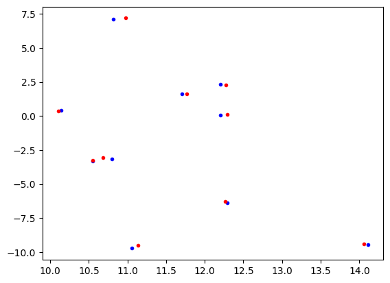
Again we can access all the information for a single sample. Here we see the full state tracked by the system. In addition to the host and source nodes we created, the information for the functional nodes is tracked.

single_sample = state.extract_single_sample(0)
print(str(single_sample))

NumpyRandomFunc:uniform_3:
    low: 10.0
    high: 15.0
    function_node_result: 13.67724606381481
host:
    ra: 13.67724606381481
    dec: -5.879624849547729
    redshift: None
    t0: None
    distance: None
    brightness: 15.0
NumpyRandomFunc:uniform_4:
    low: -10.0
    high: 10.0
    function_node_result: -5.879624849547729
NumpyRandomFunc:normal_1:
    loc: 13.67724606381481
    scale: 0.1
    function_node_result: 13.614762339036108
source:
    ra: 13.614762339036108
    dec: -5.978136502822448
    redshift: None
    t0: None
    distance: None
    brightness: 100.0
NumpyRandomFunc:normal_5:
    loc: -5.879624849547729
    scale: 0.1
    function_node_result: -5.978136502822448

It is interesting to note that functional nodes themselves are parameterized nodes, allowing for more complex forms of chaining. For example we could set the low parameter from one of the NumpyRandomFuncs from another function node. This allows us to specify priors and comlex distributions.

Similarly we can now make the input parameters of one node depend on a function of parameters from other nodes. We can arbitrarily chain the computations.

# Create a host galaxy with a random brightness.
host = ConstantSEDModel(
    brightness=NumpyRandomFunc("uniform", low=1.0, high=5.0),
    node_label="host",
)

# Create the brightness of the source as a uniformly sampled foreground brightness
# added to the 80% of the host's brightness (background).
source_brightness = BasicMathNode(
    "0.8 * val1 + val2",
    val1=host.brightness,
    val2=NumpyRandomFunc("uniform", low=1.0, high=2.0),
    node_label="plus_80percent",
)

source = ConstantSEDModel(
    brightness=source_brightness,
    node_label="source",
)
state = source.sample_parameters(num_samples=10)
print(f"Host Brightness: {state['host']['brightness']}")
print(f"Source Brightness: {state['source']['brightness']}")

Host Brightness: [4.36712249 1.12376298 3.67634326 3.49861059 2.67209912 4.48558216
 2.05111777 2.806384   4.99424824 4.09063482]
Source Brightness: [4.57140308 2.32531128 4.77634247 3.90767396 3.25415562 4.94457356
 3.16110956 3.92473779 5.36013873 5.05935097]

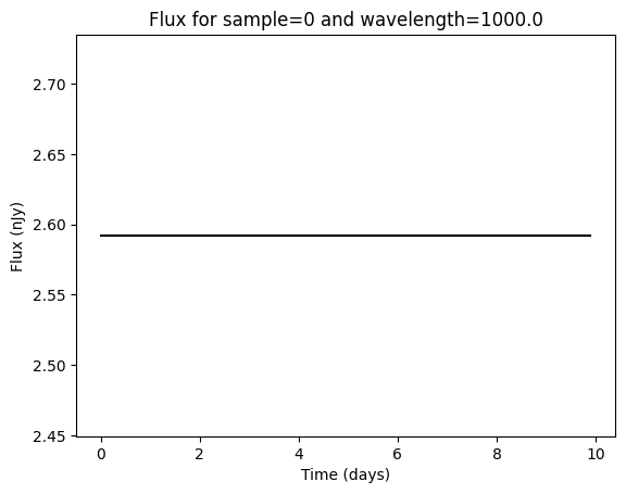
The state is used within the evaluate_sed() function to generate the flux densities.

time = np.arange(0, 10, 0.1)
waves = np.array([1000.0, 2000.0])
fluxes = source.evaluate_sed(time, waves, state)
print(f"Generated {fluxes.shape} fluxes (samples x times x wavelengths).")

# Plot the the flux for sample=0 and wavelength=1000.0.
plt.plot(time, fluxes[0, :, 0], "k-")
plt.xlabel("Time (days)")
plt.ylabel("Flux (nJy)")
plt.title("Flux for sample=0 and wavelength=1000.0")
plt.show()

Generated (10, 100, 2) fluxes (samples x times x wavelengths).

MultiObjectModels

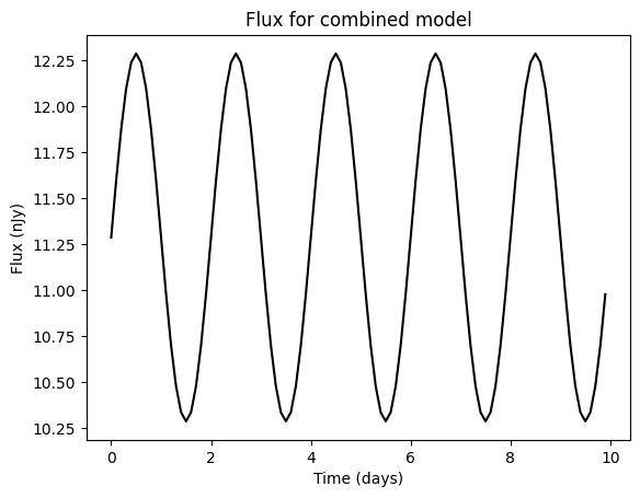
We expect that many users will want to simulate fluxes produced by a combination of objects, such as a supernova and its host galaxy. LightCurveLynx provides the AdditiveMultiObjectModel for computing such combinations. The flux produced by the model is the (weighted) sum of fluxes from the individual sources.

Each underlying model in the AdditiveMultiObjectModel separately applies rest frame effects to its component flux. This allows users to model unresolved objects at different distances (with different redshifts or dust extinctions). All observer frame effects are applied to the summed fluxes for consistency.

from lightcurvelynx.models.basic_models import SinWaveModel
from lightcurvelynx.models.multi_object_model import AdditiveMultiObjectModel

# We model the host as a galaxy with a random brightness and position.
host = ConstantSEDModel(
    brightness=NumpyRandomFunc("normal", loc=10.0, scale=1.0),
    ra=NumpyRandomFunc("uniform", low=10.0, high=15.0),
    dec=NumpyRandomFunc("uniform", low=-10.0, high=10.0),
    node_label="host",
)

# We model the source as a sine wave with a given frequency and amplitude.
source = SinWaveModel(
    brightness=1.0,
    amplitude=1.0,
    frequency=0.5,
    ra=NumpyRandomFunc("normal", loc=host.ra, scale=0.1),
    dec=NumpyRandomFunc("normal", loc=host.dec, scale=0.1),
    t0=0.0,
    node_label="sin_wave_source",
)

# We combine the host and source into a multi-source model and sample it.
combined = AdditiveMultiObjectModel(
    objects=[host, source],
    node_label="combined_model",
)
state = combined.sample_parameters(num_samples=1)
print(state)

NumpyRandomFunc:uniform_2:
    low: 10.0
    high: 15.0
    function_node_result: 11.105771576032046
host:
    ra: 11.105771576032046
    dec: -0.5459090753717994
    redshift: None
    t0: None
    distance: None
    brightness: 11.727022303141384
NumpyRandomFunc:uniform_3:
    low: -10.0
    high: 10.0
    function_node_result: -0.5459090753717994
NumpyRandomFunc:normal_4:
    loc: 10.0
    scale: 1.0
    function_node_result: 11.727022303141384
NumpyRandomFunc:normal_6:
    loc: 11.105771576032046
    scale: 0.1
    function_node_result: 11.11399129373992
sin_wave_source:
    ra: 11.11399129373992
    dec: -0.4441171549978646
    redshift: None
    t0: 0.0
    distance: None
    brightness: 1.0
    amplitude: 1.0
    frequency: 0.5
NumpyRandomFunc:normal_7:
    loc: -0.5459090753717994
    scale: 0.1
    function_node_result: -0.4441171549978646
combined_model:
    ra: None
    dec: None
    redshift: None
    t0: None
    distance: None

# Evaluate and generate the fluxes from the combined model for a
# single wavelength parameter sample.
time = np.arange(0, 10, 0.1)
fluxes = combined.evaluate_sed(time, np.array([1000.0]), state)

# Plot the the flux for sample=0 and wavelength=1000.0.
plt.plot(time, fluxes[:, 0], "k-")
plt.xlabel("Time (days)")
plt.ylabel("Flux (nJy)")
plt.title("Flux for combined model")
plt.show()