CCD-Level ObsTables

This notebook describes how to load and use survey data that is provided at a CCD level. While using CCD-level data provides additional complexities, it can allow more accurate simulation by simulating finer grained noise characteristics.

In this notebook we use a subsampling of the Rubin DP1 CCDVisit table. This data is included in LightCurveLynx’s github with the testing data.

Loading The (Subsampled) DP1 CCDVisits

We start by loading the subsample of the DP1 CCDVisits from the testing directory. As you can see from the first 5 rows of the loaded table, the times (expMidptMJD) are all identical. This is because each row represents a single CCD at a single time.

import matplotlib.pyplot as plt
import numpy as np
import pandas as pd

# We provide a relative path so the notebook renders on readthedocs. In practice, you would
# load the table from your local filesystem or a remote source.
table_file = "../../tests/lightcurvelynx/data/dp1_ccdvisit_subsampled.parquet"
pdf = pd.read_parquet(table_file)

pdf.head()

	ccdVisitId	expMidptMJD	ra	dec	band	skyRotation	magLim	seeing	skyBg	skyNoise	pixelScale	xSize	ySize	zeroPoint
9	1145019889152	60623.259329	53.004909	-28.191185	r	102.799341	24.5735	0.896197	889.033020	32.938400	0.200393	4071	3999	32.071701
10	1145019889153	60623.259329	53.064737	-27.962022	r	102.799341	24.6319	0.873288	904.945984	29.584101	0.200324	4071	3999	32.073002
11	1145019889154	60623.259329	53.124301	-27.732423	r	102.799341	24.6158	0.898227	886.961975	31.682600	0.200390	4071	3999	32.072102
12	1145019889155	60623.259329	53.265134	-28.243372	r	102.799341	24.6035	0.903278	884.517029	32.218601	0.200328	4071	3999	32.071098
13	1145019889156	60623.259329	53.324200	-28.014305	r	102.799341	24.6334	0.889979	896.465027	32.111099	0.200265	4071	3999	32.073200

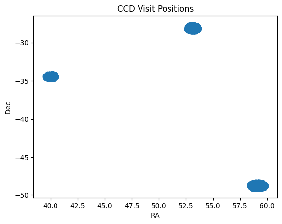
We can plot all of the pointings (all CCDs, all times).

_ = plt.scatter(pdf["ra"], pdf["dec"])
plt.xlabel("RA")
plt.ylabel("Dec")
plt.title("CCD Visit Positions")
plt.show()

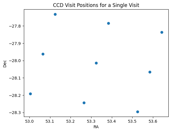
We can also look at the pointings for a single time step. Here we see nine coordinates denoting the center of each CCD.

first_time_inds = np.abs(pdf["expMidptMJD"] - 60623.259329) < 1e-6
one_timestep_pdf = pdf[first_time_inds]

_ = plt.scatter(one_timestep_pdf["ra"], one_timestep_pdf["dec"])
plt.xlabel("RA")
plt.ylabel("Dec")
plt.title("CCD Visit Positions for a Single Visit")
plt.show()

CCDs without Detector Footprints

By default ObsTable will use a circular radius to determine which points fall within the viewing area of each pointing. While this is a fast and reasonable approximation for full images (all CCDs), it can lead to problems when the pointings are provided on a per-CCD level.

To see this, let’s load our single time step into an LSSTObsTable with make_detector_footprint set to False. Note that this will give us a warning because we are loading CCD-level information.

from lightcurvelynx.obstable.lsst_obstable import LSSTObsTable

obs_table = LSSTObsTable.from_ccdvisit_table(one_timestep_pdf, make_detector_footprint=False)

/home/docs/checkouts/readthedocs.org/user_builds/lightcurvelynx/envs/stable/lib/python3.12/site-packages/lightcurvelynx/obstable/lsst_obstable.py:288: UserWarning: Not creating a detector footprint for a CCD pointing table. This may lead to duplicate results for points near the edges of the CCDs.
  warnings.warn(

Now we look at a grid of (RA, Dec) points to see which ones are observed. The range_search() function is what LightCurveLynx’s simulation uses to determine when each sampled (RA, Dec) is observed.

ra, dec = np.meshgrid(np.linspace(52.5, 54, 50), np.linspace(-27.5, -28.5, 50))
ra = ra.flatten()
dec = dec.flatten()

# Find the matches with the default radius for an LSST CCD, which is ~0.1574 degrees.
matching_inds = obs_table.range_search(ra, dec)
num_matches = np.array([len(matches) for matches in matching_inds])

for count in np.unique(num_matches):
    print(f"Number of points with {count} matches: {(num_matches == count).sum()}")

    plt.scatter(ra[num_matches == count], dec[num_matches == count], label=f"{count} matches")

plt.xlabel("RA")
plt.ylabel("Dec")
plt.title("CCD Visit Positions for a Single Visit")
plt.legend()
plt.show()

Number of points with 0 matches: 1470
Number of points with 1 matches: 781
Number of points with 2 matches: 249

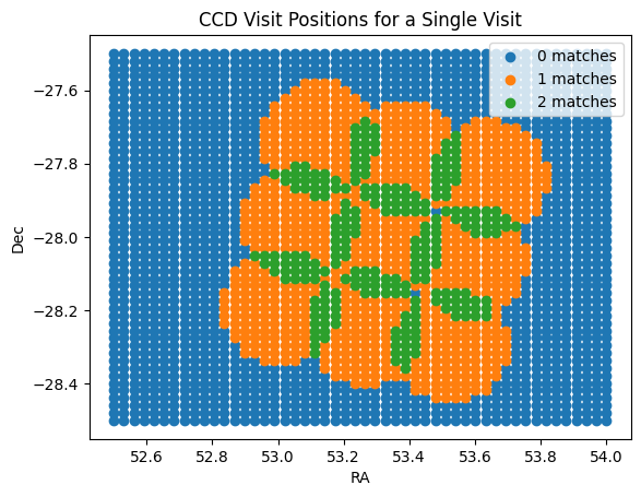
As we can see, a fair number of points are observed multiple times. This is incorrect and an artifact of using a circular radius. In reality, each point will only be observed by a single CCD.

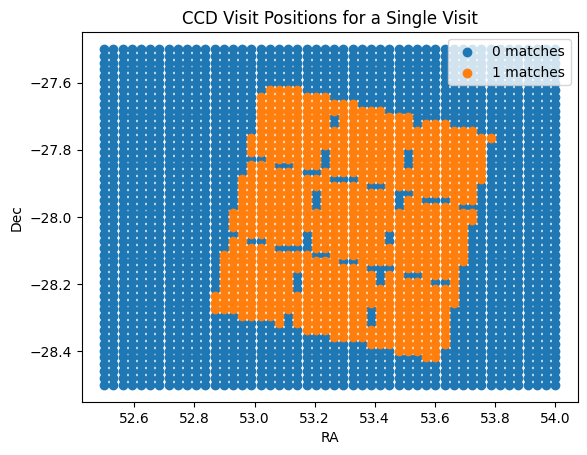
CCDs with Detector Footprints

The ObsTable has the ability to use a detector footprint in the range search. While you can manually set a detector footprint, the LSSTObsTable.from_ccdvisit_table can also automatically generate one from the known information about Rubin’s CCDs. For more information on detector footprints, see the detector footprint notebook.

When we rerun the range search, we now see the expected behavior. We even see chip gaps!

obs_table2 = LSSTObsTable.from_ccdvisit_table(one_timestep_pdf, make_detector_footprint=True)

# Find the matches with the default radius for an LSST CCD, which is ~0.1574 degrees.
matching_inds = obs_table2.range_search(ra, dec)
num_matches = np.array([len(matches) for matches in matching_inds])

for count in np.unique(num_matches):
    print(f"Number of points with {count} matches: {(num_matches == count).sum()}")

    plt.scatter(ra[num_matches == count], dec[num_matches == count], label=f"{count} matches")

plt.xlabel("RA")
plt.ylabel("Dec")
plt.title("CCD Visit Positions for a Single Visit")
plt.legend()
plt.show()

Number of points with 0 matches: 1694
Number of points with 1 matches: 806

Conclusion

When simulating from CCD-level pointing information, users will almost always want to apply a detector footprint.