Saturation
This notebook describes how saturation is handled during simulation.
The ObsTable class provides an option to define saturation thresholds in each band (in magnitudes). If provided, these saturation thresholds are applied during the simulation step.
Setup
We start by loading the survey data needed to perform a simulation: the observation table and the passbands. For the passbands, we use the LSST preset. However, for the survey pointings, we generate artificial data that will help us visualize the impact. We pick a single pointing (RA=0, dec=-10.0) and 100 days of evenly sampled data in four alternating bands.
Note that the OpSim uses the expected LSST saturation thresholds by default. In fact most survey types will have these thresholds predefined. We overwrite the saturation thresholds with given values.
[1]:
import numpy as np

from lightcurvelynx.astro_utils.passbands import PassbandGroup
from lightcurvelynx.astro_utils.mag_flux import mag2flux
from lightcurvelynx.obstable.opsim import OpSim
from lightcurvelynx.survey_info import SurveyInfo


# Usually we would not hardcode the path to the passband files, but for this demo we will use a relative path
# to the test data directory so that we do not have to download the files.
table_dir = "../../tests/lightcurvelynx/data/passbands"
passband_group = PassbandGroup.from_preset(preset="LSST", table_dir=table_dir)

# Generate fake observation data for testing.
num_times = 200
times = 60676.0 + np.arange(num_times) * 0.25  # 200 observations spaced 0.25 days apart
obsdata = {
    "time": times,
    "ra": np.full(num_times, 0.0),
    "dec": np.full(num_times, -10.0),
    "filter": np.tile(["r", "g", "i", "z"], num_times // 4),
    "zp": np.full(num_times, 1.0),
    "seeing": np.full(num_times, 1.12),
    "skybrightness": np.full(num_times, 24.0),
    "exptime": np.full(num_times, 15.0),
    "nexposure": np.full(num_times, 2),
}

# Define saturation thresholds for each passband. These are not the actual LSST saturation thresholds,
# but exagerated values for demonstration purposes.
saturation_thresholds = {
    "u": 14.0,
    "g": 15.0,
    "r": 16.0,
    "i": 17.0,
    "z": 22.0,
    "y": 19.0,
}
for f, lim in saturation_thresholds.items():
    print(f"Saturation threshold for {f}-band: {lim} mag = {mag2flux(lim):.2e} nJy")

opsim = OpSim(obsdata, saturation_mags=saturation_thresholds)
print(f"Created OpSim with {len(opsim)} observations.")

survey_info = SurveyInfo(obstable=opsim, passbands=passband_group, survey_name="LSST")
/home/docs/checkouts/readthedocs.org/user_builds/lightcurvelynx/envs/latest/lib/python3.12/site-packages/tqdm/auto.py:21: TqdmWarning: IProgress not found. Please update jupyter and ipywidgets. See https://ipywidgets.readthedocs.io/en/stable/user_install.html
  from .autonotebook import tqdm as notebook_tqdm
Saturation threshold for u-band: 14.0 mag = 9.12e+06 nJy
Saturation threshold for g-band: 15.0 mag = 3.63e+06 nJy
Saturation threshold for r-band: 16.0 mag = 1.45e+06 nJy
Saturation threshold for i-band: 17.0 mag = 5.75e+05 nJy
Saturation threshold for z-band: 22.0 mag = 5.75e+03 nJy
Saturation threshold for y-band: 19.0 mag = 9.12e+04 nJy
Created OpSim with 200 observations.
Model
To demonstrate the impact of saturation thresholds, we define a simple model with brightness that is maximum at t0. While not realistic, this model is useful for the visualization we will want to do.
[2]:
import numpy as np

from lightcurvelynx.models.physical_model import SEDModel
from lightcurvelynx.astro_utils.mag_flux import mag2flux


class PeakedModel(SEDModel):
    """A model that starts at a base brightness, increases linearly
    to t0, and then decreases linearly after t0 back to the base brightness.

    Parameters
    ----------
    base : parameter
        The base brightness in nJy.
    peak : parameter
        The peak brightness in nJy at time t0.
    slope : parameter
        The slope of the linear function in nJy/day.
    **kwargs : dict, optional
        Any additional keyword arguments.
    """

    def __init__(self, base, peak, slope, **kwargs):
        super().__init__(**kwargs)
        self.add_parameter("base", base, **kwargs)
        self.add_parameter("peak", peak, **kwargs)
        self.add_parameter("slope", slope, **kwargs)

    def compute_sed(self, times, wavelengths, graph_state, **kwargs):
        """Draw effect-free observations for this object.

        Parameters
        ----------
        times : numpy.ndarray
            A length T array of rest frame timestamps.
        wavelengths : numpy.ndarray, optional
            A length N array of wavelengths (in angstroms).
        graph_state : GraphState
            An object mapping graph parameters to their values.
        **kwargs : dict, optional
            Any additional keyword arguments.

        Returns
        -------
        flux_density : numpy.ndarray
            A length T x N matrix of SED values (in nJy).
        """
        params = self.get_local_params(graph_state)
        linear_function = params["peak"] - params["slope"] * np.abs(times - params["t0"])
        single_wave = np.maximum(params["base"], linear_function)
        return np.tile(single_wave[:, np.newaxis], (1, len(wavelengths)))


# Create a model instance with a base brightness of 20 mag,
# a peak brightness of 12 mag, and a slope of 1 magnitude/day.
model = PeakedModel(
    base=mag2flux(20.0),  # Base brightness of 20 mag
    peak=mag2flux(15.0),  # Peak brightness of 15 mag
    slope=200_000.0,  # Slope of 10000 nJy/day (exagerated for demonstration)
    ra=0.0,
    dec=-10.0,
    t0=60700.0,
    redshift=1e-8,
)
Running the Simulation
We start by running the simulation for the model with no saturation. Since the OpSim has saturation thresholds provided, we control this by using the apply_saturation flag in simulation function.
[3]:
from lightcurvelynx.simulate import simulate_lightcurves
from lightcurvelynx.utils.plotting import plot_lightcurves

results_no_sat = simulate_lightcurves(model, 1, survey_info, apply_saturation=False)

# Plot the resulting lightcurve.
lc = results_no_sat.loc[0]["lightcurve"]
filters = np.asarray(lc["filter"], dtype=str)
_ = plot_lightcurves(
    fluxes=np.asarray(lc["flux"], dtype=float),
    times=np.asarray(lc["mjd"], dtype=float),
    filters=filters,
)
Simulating: 100%|██████████| 1/1 [00:00<00:00, 369.44obj/s]
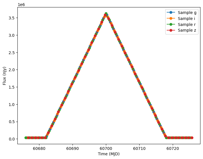
As we can see from the plot the simulated bandflux for each filter peaks at the same level.
The simulation also sets a “is_saturated” for each observation in the light curve. Nothing is marked as saturated.
[4]:
for filter_name in np.unique(filters):
    filter_count = (filters == filter_name).sum()
    saturated_count = ((filters == filter_name) & lc["is_saturated"]).sum()
    print(
        f"Number of saturated points in {filter_name}-band: {saturated_count} of {filter_count} total points"
    )
Number of saturated points in g-band: 0 of 50 total points
Number of saturated points in i-band: 0 of 50 total points
Number of saturated points in r-band: 0 of 50 total points
Number of saturated points in z-band: 0 of 50 total points
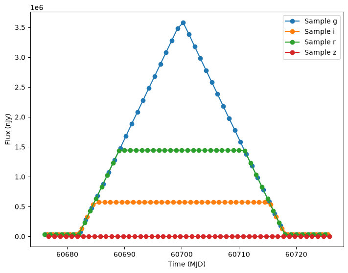
Now we rerun the simulation with saturation enabled (by leaving off the flag). We see the filters peak at different levels and have different numbers of points marked as saturated.
[5]:
results_sat = simulate_lightcurves(model, 1, opsim, passband_group)

# Plot the resulting lightcurve.
lc = results_sat.loc[0]["lightcurve"]
_ = plot_lightcurves(
    fluxes=np.asarray(lc["flux"], dtype=float),
    times=np.asarray(lc["mjd"], dtype=float),
    filters=np.asarray(lc["filter"], dtype=str),
)

for filter_name in np.unique(filters):
    filter_count = (filters == filter_name).sum()
    saturated_count = ((filters == filter_name) & lc["is_saturated"]).sum()
    print(
        f"Number of saturated points in {filter_name}-band: {saturated_count} of {filter_count} total points"
    )
/home/docs/checkouts/readthedocs.org/user_builds/lightcurvelynx/envs/latest/lib/python3.12/site-packages/lightcurvelynx/simulate.py:716: FutureWarning: The passbands argument is deprecated and will be removed from future versions.
  warnings.warn(
/home/docs/checkouts/readthedocs.org/user_builds/lightcurvelynx/envs/latest/lib/python3.12/site-packages/lightcurvelynx/simulate.py:728: FutureWarning: Passing ObsTable objects directly in survey_info is deprecated and will be removed in future versions. Please use SurveyInfo objects instead.
  warnings.warn(
Simulating: 100%|██████████| 1/1 [00:00<00:00, 556.72obj/s]
Number of saturated points in g-band: 0 of 50 total points
Number of saturated points in i-band: 30 of 50 total points
Number of saturated points in r-band: 21 of 50 total points
Number of saturated points in z-band: 50 of 50 total points