Working with Rubin CCDVisit Table Data

In this notebook we look at how we can import data from the Rubin CCDVisit table such as DP1, the Science Validation DB or DP2 CCDVisits Table. The observed LSST data uses the LSSTObsTable class instead of the OpSim class (which should only be used for simulated data).

Note that the lsst packages are not installed as part of the default LightCurveLynx installation. Users will need to manually install them via in order to run this notebook (e.g. pip install lsst-rsp)

Get the Visits Table

Users will need to download the CCDVisits table. Here we use the parquet version of the DP1 ccdvisits table on LSDB.io. This notebook assumes the table has been downloaded to a local directory. A subsampled copy of this data is also included in the lightcurvelynx repository at: “tests/lightcurvelynx/data/dp1_ccdvisit_subsampled.parquet”.

import pandas as pd

filename = "../../../data/opsim/dp1_ccdvisit.parquet"
survey_data = pd.read_parquet(filename)
survey_data.head()

	ccdVisitId	expMidptMJD	ra	dec	band	skyRotation	magLim	seeing	skyBg	skyNoise	pixelScale	xSize	ySize	zeroPoint
0	1145019888896	60623.258521	53.004536	-28.190331	i	102.799379	24.1963	0.864554	1425.880005	40.683998	0.200343	4071	3999	31.839001
1	1145019888897	60623.258521	53.064355	-27.961231	i	102.799379	24.2392	0.823865	1422.500000	37.339401	0.200280	4071	3999	31.838699
2	1145019888898	60623.258521	53.123909	-27.731684	i	102.799379	24.2087	0.844020	1418.369995	39.185101	0.200342	4071	3999	31.836599
3	1145019888899	60623.258521	53.264695	-28.242508	i	102.799379	24.1806	0.859669	1425.849976	39.428398	0.200274	4071	3999	31.837999
4	1145019888900	60623.258521	53.323752	-28.013505	i	102.799379	24.2486	0.808050	1424.319946	39.147900	0.200218	4071	3999	31.839100

Creating the ObsTable

The LSSTObsTable class includes a method for building an ObsTable directly from a Rubin CCDVisists table. It includes the schemas for both DP1 and DP2 data.

Note that the CCDVisits table provides one pointing per-ccd. If you do not use a detector footprint (and fallback to a circular areas), the same sampled point can get picked up by multiple CCDs. This will show up as multiple points in the light curve having the same time stamp and filter

We will get an expected warning from the fact that the DP1 CCDVisits table has NaNs in some of the noise columns.

from lightcurvelynx.obstable.lsst_obstable import LSSTObsTable

obs_table = LSSTObsTable.from_ccdvisit_table(survey_data, make_detector_footprint=True)

/Users/jkubica/h/lightcurvelynx/src/lightcurvelynx/obstable/lsst_obstable.py:251: UserWarning: Found NaN values in critical column 'seeing'. Dropping rows with NaN values in this column.
  warnings.warn(

This means that the function will automatically handle translating the column names to those expected by LightCurveLynx. By comparing the column names, we can see some of the renaminings (e.g. “band” -> “filter”)

cols1 = set(obs_table.columns.tolist())
cols2 = set(survey_data.columns.tolist())

print("Columns dropped from survey_data to obs_table:")
print(cols2 - cols1)

print("Columns added to obs_table from defaults or calculations:")
print(cols1 - cols2)

Columns dropped from survey_data to obs_table:
{'magLim', 'zeroPoint', 'expMidptMJD', 'skyRotation', 'band', 'skyBg', 'pixelScale'}
Columns added to obs_table from defaults or calculations:
{'radius', 'sky_bg_e', 'maglim', 'zp_mag_adu', 'time', 'sky_bg_adu', 'zp', 'psf_footprint', 'filter', 'rotation', 'pixel_scale'}

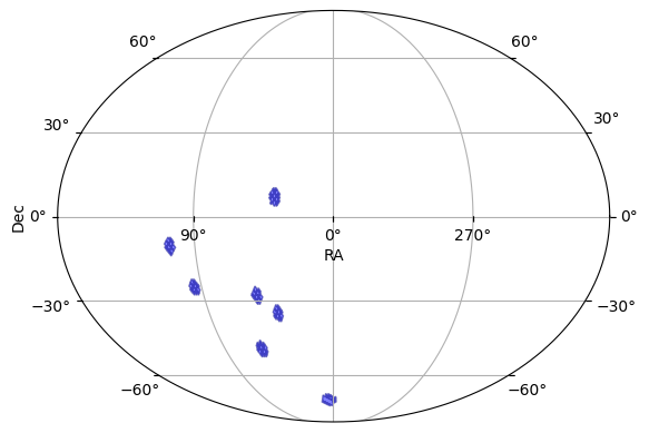
We can plot the footprint of the survery using the plot_footprint function. Since we are only looking at the entire survey coverage, we do not plot the MOC at the detector level.

obs_table.plot_footprint(use_footprint=False)

(<Figure size 640x480 with 1 Axes>, <WCSAxes: >)

Science Validation Table

The LSSTObsTable class also includes methods for reading from the database of science validation information. This database uses a columns that are a combination of those defined in the Rubin OpSim tables and the ConsDB table. The loader function automatically handles the column mapping.

This notebook assumes the lsstcam_20250930.db science validation table has already been downloaded to a local directory. We use LightCurveLynx’s read_sqlite_table to load the table.

from lightcurvelynx.utils.io_utils import read_sqlite_table

filename2 = "../../../data/opsim/lsstcam_20250930.db"
table = read_sqlite_table(filename2, sql_query="SELECT * FROM observations")

obs_table2 = LSSTObsTable.from_sv_visits_table(table)

print(f"Loaded {len(obs_table2)} observations from {filename2}")
print("Columns in obs_table2:")
print(obs_table2.columns.tolist())

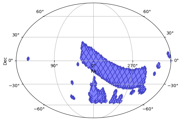
obs_table2.plot_footprint()

/Users/jkubica/h/lightcurvelynx/src/lightcurvelynx/obstable/lsst_obstable.py:319: UserWarning: Found NaN values in critical columns ['sky_bg_median', 'zero_point_median']. Dropping rows with NaN values in these columns.
  warnings.warn(

Loaded 20436 observations from ../../../data/opsim/lsstcam_20250930.db
Columns in obs_table2:
['observationId', 'exposure_name', 'controller', 'day_obs', 'seq_num', 'physical_filter', 'filter', 'ra', 'dec', 'rotation', 'azimuth_start', 'azimuth_end', 'azimuth', 'altitude_start', 'altitude_end', 'altitude', 'zenith_distance_start', 'zenith_distance_end', 'zenith_distance', 'airmass', 'exp_midpt', 'time', 'obs_start', 'observationStartMJD', 'obs_end', 'obs_end_mjd', 'exptime', 'shut_time', 'visitTime', 'group_id', 'cur_index', 'max_index', 'img_type', 'emulated', 'science_program', 'observation_reason', 'target_name', 'air_temp', 'pressure', 'humidity', 'wind_speed', 'wind_dir', 'dimm_seeing', 'focus_z', 'simulated', 'vignette', 'vignette_min', 'scheduler_note', 's_region', 'can_see_sky', 'n_inputs', 'pixel_scale_min', 'pixel_scale_max', 'pixel_scale_median', 'astrom_offset_mean_min', 'astrom_offset_mean_max', 'astrom_offset_mean_median', 'astrom_offset_std_min', 'astrom_offset_std_max', 'astrom_offset_std_median', 'eff_time_min', 'eff_time_max', 'eff_time_median', 'eff_time_psf_sigma_scale_min', 'eff_time_psf_sigma_scale_max', 'eff_time_psf_sigma_scale_median', 'eff_time_sky_bg_scale_min', 'eff_time_sky_bg_scale_max', 'eff_time_sky_bg_scale_median', 'eff_time_zero_point_scale_min', 'eff_time_zero_point_scale_max', 'eff_time_zero_point_scale_median', 'stats_mag_lim_min', 'stats_mag_lim_max', 'stats_mag_lim_median', 'psf_ap_flux_delta_min', 'psf_ap_flux_delta_max', 'psf_ap_flux_delta_median', 'psf_ap_corr_sigma_scaled_delta_min', 'psf_ap_corr_sigma_scaled_delta_max', 'psf_ap_corr_sigma_scaled_delta_median', 'max_dist_to_nearest_psf_min', 'max_dist_to_nearest_psf_max', 'max_dist_to_nearest_psf_median', 'mean_var_min', 'mean_var_max', 'mean_var_median', 'n_psf_star_min', 'n_psf_star_max', 'n_psf_star_median', 'n_psf_star_total', 'psf_area_min', 'psf_area_max', 'psf_area_median', 'psf_ixx_min', 'psf_ixx_max', 'psf_ixx_median', 'psf_ixy_min', 'psf_ixy_max', 'psf_ixy_median', 'psf_iyy_min', 'psf_iyy_max', 'psf_iyy_median', 'psf_sigma_min', 'psf_sigma_max', 'psf_sigma_median', 'psf_star_delta_e1_median_min', 'psf_star_delta_e1_median_max', 'psf_star_delta_e1_median_median', 'psf_star_delta_e1_scatter_min', 'psf_star_delta_e1_scatter_max', 'psf_star_delta_e1_scatter_median', 'psf_star_delta_e2_median_min', 'psf_star_delta_e2_median_max', 'psf_star_delta_e2_median_median', 'psf_star_delta_e2_scatter_min', 'psf_star_delta_e2_scatter_max', 'psf_star_delta_e2_scatter_median', 'psf_star_delta_size_median_min', 'psf_star_delta_size_median_max', 'psf_star_delta_size_median_median', 'psf_star_delta_size_scatter_min', 'psf_star_delta_size_scatter_max', 'psf_star_delta_size_scatter_median', 'psf_star_scaled_delta_size_scatter_min', 'psf_star_scaled_delta_size_scatter_max', 'psf_star_scaled_delta_size_scatter_median', 'psf_trace_radius_delta_min', 'psf_trace_radius_delta_max', 'psf_trace_radius_delta_median', 'sky_bg_min', 'sky_bg_max', 'sky_bg_e', 'sky_noise_min', 'sky_noise_max', 'sky_noise_median', 'seeing_zenith_500nm_min', 'seeing_zenith_500nm_max', 'seeing_zenith_500nm_median', 'zero_point_min', 'zero_point_max', 'zp_mag_e', 'low_snr_source_count_min', 'low_snr_source_count_max', 'low_snr_source_count_median', 'low_snr_source_count_total', 'high_snr_source_count_min', 'high_snr_source_count_max', 'high_snr_source_count_median', 'high_snr_source_count_total', 'z4', 'z5', 'z6', 'z7', 'z8', 'z9', 'z10', 'z11', 'z12', 'z13', 'z14', 'z15', 'z16', 'z17', 'z18', 'z19', 'z20', 'z21', 'z22', 'z23', 'z24', 'z25', 'z26', 'z27', 'z28', 'ringss_seeing', 'aos_fwhm', 'donut_blur_fwhm', 'physical_rotator_angle', 'prev_obs_start_mjd', 'prev_obs_end_mjd', 'slewTime', 'eclip_lat', 'eclip_lon', 'gal_lat', 'gal_lon', 'seeing', 'seeingFwhmGeom', 'FWHM_500', 'lst', 'HA', 'approx_pa', 'approx_rotTelPos', 'moonAlt', 'moonAz', 'moonRA', 'moonDec', 'moonDistance', 'moonPhase', 'sunAlt', 'sunAz', 'sunRA', 'sunDec', 'zero_point_1s', 'zero_point_1s_pred', 'cloud_extinction', 'sky_bg_mag', 'maglim', 'slew_model', 'slew_model_ideal', 'model_gap', 'slewDistance', 'overhead', 'fault', 'jd', 'nexp', 'night', 'zp', 'psf_footprint']

(<Figure size 640x480 with 1 Axes>, <WCSAxes: >)

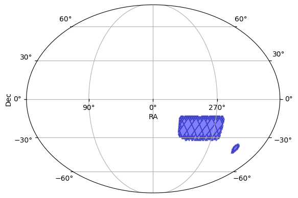
A highly subsampled copy of this data is also included locally in “tests/lightcurvelynx/data/sv_db_subsampled.db”.

from lightcurvelynx import _LIGHTCURVELYNX_TEST_DATA_DIR

filename2 = "../../../data/opsim/lsstcam_20250930.db"
table = read_sqlite_table(
    _LIGHTCURVELYNX_TEST_DATA_DIR / "sv_db_subsampled.db",
    sql_query="SELECT * FROM observations",
)

obs_table3 = LSSTObsTable.from_sv_visits_table(table)

print(f"Loaded {len(obs_table3)} observations from {filename2}")
print("Columns in obs_table3:")
print(obs_table3.columns.tolist())

obs_table3.plot_footprint()

Loaded 4045 observations from ../../../data/opsim/lsstcam_20250930.db
Columns in obs_table3:
['index', 'filter', 'ra', 'dec', 'rotation', 'time', 'exptime', 'sky_bg_e', 'zp_mag_e', 'seeing', 'maglim', 'zp', 'psf_footprint']

(<Figure size 640x480 with 1 Axes>, <WCSAxes: >)

Conclusion

The LSSTObsTable created from the CCDVisits table or science validation DB can be used like any other ObsTable.