Parameter Sampling with Modeldag

This notebook demonstrates how users can employ Mickael Rigault’s powerful and flexible modeldag package for statistical sampling. The modeldag package functions similarly to LightCurveLynx’s internal sampling package, by defining a directed acyclic graph of parameters that are generated from each other. Users should be able to convert back and forth between the two. However, we provide a direct wrapper to modeldag in case users are more familiar with it, want to define the DAG in a single dictionary, or want to make use of the package’s additional helper functions.

Note that the modeldag is not installed as part of the default LightCurveLynx installation. Users will need to manually install pzflow via pip (e.g. pip install modeldag) in order to run this notebook.

Introduction to modeldag

The modeldag package provides a user-friendly framework for defining directed acyclic graphs of parameters. The entire graph is specified in a dictionary where the keys are the parameters to be sampled. The values contain information need to sample. The most common formulation of a value is another dictionary that includes the following information:

• func: The function that will be used to set this parameter.

• kwargs: Another dictionary where the keys are the input parameters and the values are the their inputs.

For example if we want a single parameter a sampled from a numpy normal distribution with mean=10 and standard deviation=2, we could specify the model as:

import numpy as np
import modeldag

dag_dict = {
    "a": {"func": np.random.normal, "kwargs": {"loc": 10, "scale": 2}},
}
model = modeldag.ModelDAG(dag_dict)

model.draw(100).head()

	a
0	9.726262
1	11.092842
2	11.777541
3	13.316172
4	6.537147

The power of the modeldag package is that you can use the @ notation to chain parameter dependencies. For example, we can define a second parameter b as being sampled from a distribution that depends on the value of the a parameter. In this case we first sample a and then sample b from a normal distribution centered on a.

dag_dict = {
    "a": {"func": np.random.normal, "kwargs": {"loc": 10, "scale": 2}},
    "b": {"func": np.random.normal, "kwargs": {"loc": "@a", "scale": 1}},
}
model = modeldag.ModelDAG(dag_dict)

model.draw(100).head()

	a	b
0	9.726262	9.784952
1	11.092842	10.829707
2	11.777541	11.754535
3	13.316172	13.910843
4	6.537147	7.709241

The ModelDAGNode

LightCurveLynx provides a ModelDAGNode node to wrap modeldag.ModelDAG. Sampling this node samples all the parameters at once and makes them available via LightCurveLynx’s dot notation.

from lightcurvelynx.math_nodes.modeldag_node import ModelDAGNode

node = ModelDAGNode(model, node_label="test")

state = node.sample_parameters(num_samples=5)
print(state)

test:
    a: [ 8.19732958 10.39657291  8.58963686 11.25446369  9.88448502]
    b: [ 8.1330717   9.05986181  8.01389105 11.28568635  8.87300583]

This allows us to use the sampled parameters in chaining.

We can define a modeldag.ModelDAG that generates values for two parameters (a sin wave’s amplitude and frequency), then feed those into a LightCurveLynx model using the dot notation.

from lightcurvelynx.models.basic_models import SinWaveModel

dag_dict = {
    "amplitude": {"func": np.random.normal, "kwargs": {"loc": 10, "scale": 2}},
    "frequency": {"func": np.random.uniform, "kwargs": {"low": 0.1, "high": 1.0}},
}
dag_params_node = ModelDAGNode(modeldag.ModelDAG(dag_dict))

source = SinWaveModel(
    amplitude=dag_params_node.amplitude,
    frequency=dag_params_node.frequency,
    t0=0.0,
    ra=10.0,
    dec=-5.0,
    node_label="source",
)
state = source.sample_parameters(num_samples=5)
print(state)

source:
    ra: [10. 10. 10. 10. 10.]
    dec: [-5. -5. -5. -5. -5.]
    redshift: [None None None None None]
    t0: [0. 0. 0. 0. 0.]
    distance: [None None None None None]
    brightness: [0. 0. 0. 0. 0.]
    amplitude: [ 9.72626179 11.0928425  11.77754055 13.31617211  6.53714672]
    frequency: [0.56606981 0.35294526 0.39227821 0.79254678 0.67753464]
ModelDAGNode:_non_func_1:
    amplitude: [ 9.72626179 11.0928425  11.77754055 13.31617211  6.53714672]
    frequency: [0.56606981 0.35294526 0.39227821 0.79254678 0.67753464]

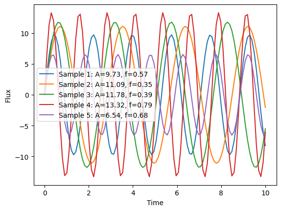
We could then use that sampling to evaluate multiple SEDs.

import matplotlib.pyplot as plt

times = np.linspace(0, 10, 100)
wavelengths = np.array([500])

fluxes = source.evaluate_sed(times, wavelengths, graph_state=state)

for i in range(5):
    amp = state["source"]["amplitude"][i]
    freq = state["source"]["frequency"][i]
    label = f"Sample {i + 1}: A={amp:.2f}, f={freq:.2f}"
    plt.plot(times, fluxes[i, :, 0], label=label)
plt.xlabel("Time")
plt.ylabel("Flux")
plt.legend()
plt.show()

A more complex example is using the same modeldag.ModelDAG to generate related parameters for a host and a source.

dag_dict = {
    "host_ra": {"func": np.random.uniform, "kwargs": {"low": 0.0, "high": 360.0}},
    "host_dec": {"func": np.random.uniform, "kwargs": {"low": -90.0, "high": 90.0}},
    "source_ra": {"func": np.random.normal, "kwargs": {"loc": "@host_ra", "scale": 0.001}},
    "source_dec": {"func": np.random.normal, "kwargs": {"loc": "@host_dec", "scale": 0.001}},
}
host_source_params = ModelDAGNode(modeldag.ModelDAG(dag_dict))

state = host_source_params.sample_parameters(num_samples=5)
print(state)

ModelDAGNode:_non_func_0:
    host_ra: [341.2899243  139.5996536  245.48920598 215.10364213  33.36435976]
    host_dec: [ 56.12035744 -16.63566961 -28.3143023    3.21396149 -39.41094735]
    source_ra: [341.29103865 139.59892897 245.48829608 215.10399262  33.36357123]
    source_dec: [ 56.11973382 -16.63564797 -28.31331627   3.21326978 -39.4106833 ]

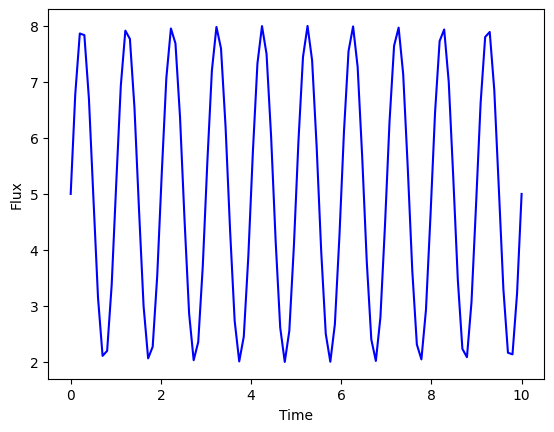
We we could feed into a combined model (for more detail on the additive models, see the Simulating Combinations of Objects notebook)

from lightcurvelynx.models.basic_models import SinWaveModel, ConstantSEDModel
from lightcurvelynx.models.multi_object_model import AdditiveMultiObjectModel

host_model = ConstantSEDModel(
    brightness=5.0,
    ra=host_source_params.host_ra,
    dec=host_source_params.host_dec,
    node_label="host",
)

source_model = SinWaveModel(
    amplitude=3.0,
    frequency=1.0,
    t0=0.0,
    ra=host_source_params.source_ra,
    dec=host_source_params.source_dec,
)

model = AdditiveMultiObjectModel(
    objects=[source_model, host_model],
    ra=source_model.ra,
    dec=source_model.dec,
    node_label="combined",
)
state = model.sample_parameters(num_samples=1)
print(state)

ModelDAGNode:_non_func_2:
    host_ra: 129.39333407664455
    host_dec: 60.15070919504622
    source_ra: 129.39224272030174
    source_dec: 60.149701686284025
SinWaveModel_1:
    ra: 129.39224272030174
    dec: 60.149701686284025
    redshift: None
    t0: 0.0
    distance: None
    brightness: 0.0
    amplitude: 3.0
    frequency: 1.0
host:
    ra: 129.39333407664455
    dec: 60.15070919504622
    redshift: None
    t0: None
    distance: None
    brightness: 5.0
combined:
    ra: 129.39224272030174
    dec: 60.149701686284025
    redshift: None
    t0: None
    distance: None

times = np.linspace(0, 10, 100)
wavelengths = np.array([500])

fluxes = model.evaluate_sed(times, wavelengths, graph_state=state)

plt.plot(times, fluxes[:, 0], color="blue")
plt.xlabel("Time")
plt.ylabel("Flux")
plt.show()