Debugging Simulations and Models
LightCurveLynx provides a variety of tools to help users understand what is happening within a simulation and how a model is working. This notebook provides an overview of some of the common approaches a user can employ to investigate model performance.
The GraphState
LightCurveLynx uses a GraphState object to store all of the information about the sampled parameters. These saved values include not only the settings of the physical object being simulated, such as its redshift, but also parameters of prior distributions and internal bookkeeping values. Thus it is a good place to inspect what is happening at different stages of your parameter graph.
Users can think of the GraphState as a nested dictionary where parameters are indexed by two levels. In the first level, the node label tells the code which object the parameter belongs to. This level of identification is necessary to allow different stages to use parameters with the same name. If we are blending many objects, we could have different RA values for each of the sources. In the second level of the GraphState, the parameter name maps to the actual sampled values.
As a concrete example, let’s look at a static object with a random parameter for brightness that is the sum of randomly chosen object brightness and background brightness.
[1]:
from lightcurvelynx.math_nodes.basic_math_node import BasicMathNode
from lightcurvelynx.math_nodes.np_random import NumpyRandomFunc
from lightcurvelynx.models.basic_models import ConstantSEDModel

obj_brightness = NumpyRandomFunc("uniform", low=1000.0, high=3000.0)
bg_brightness = NumpyRandomFunc("uniform", low=100.0, high=500.0)
total_brightness = BasicMathNode("obj + bg", obj=obj_brightness, bg=bg_brightness)

model = ConstantSEDModel(
    brightness=total_brightness,
    t0=0.0,
    ra=45.0,
    dec=-10.0,
    node_label="model",
)
/home/docs/checkouts/readthedocs.org/user_builds/lightcurvelynx/envs/latest/lib/python3.12/site-packages/tqdm/auto.py:21: TqdmWarning: IProgress not found. Please update jupyter and ipywidgets. See https://ipywidgets.readthedocs.io/en/stable/user_install.html
  from .autonotebook import tqdm as notebook_tqdm
We use the sample_parameters() function to generate a GraphState.
[2]:
state = model.sample_parameters()
print(state)
model:
    ra: 45.0
    dec: -10.0
    redshift: None
    t0: 0.0
    distance: None
    brightness: 2945.2844542690364
NumpyRandomFunc:uniform_2:
    low: 1000.0
    high: 3000.0
    function_node_result: 2802.3014697961225
BasicMathNode:eval_1:
    obj: 2802.3014697961225
    bg: 142.98298447291393
    function_node_result: 2945.2844542690364
NumpyRandomFunc:uniform_3:
    low: 100.0
    high: 500.0
    function_node_result: 142.98298447291393
Our model consists of four nodes. The top-level nodes uses numpy to generate a random brightness for the object (uniformly [1000.0, 3000.0]) and a background (uniformly [100.0, 500.0]. The second level node simply adds the two nodes together to produce a total_brightness function. The final node creates a constant SED model with the given brightness. Thus the realized brightness of the sampled object will depend on a chain of nodes and two randomly sampled parameters.
Querying Parameters
Once a user has a node, they might be interested in the full set of parameters that can be set within this node. This is particular important when dealing with nodes for physical objects where parameters maybe be added by a chain of subclasses. For example, the EclipsingBinaryStar is a subclass of PeriodicVariableStar which is a subclass of PeriodicModel which is a subclass of SEDModel and so on. Any of those classes can add its own parameters.
Users can retrieve a list of the parameters for a node:
[3]:
model.list_params()
[3]:
['ra', 'dec', 'redshift', 't0', 'distance', 'brightness']
or print out expanded descriptions:
[4]:
model.describe_params()
Parameters in model:

ra:
    Description: The object's right ascension (in degrees)
    Source: CONSTANT with value = 45.0

dec:
    Description: The object's declination (in degrees)
    Source: CONSTANT with value = -10.0

redshift:
    Description: The object's redshift.
    Source: CONSTANT with value = None

t0:
    Description: The phase offset in MJD.
    Source: CONSTANT with value = 0.0

distance:
    Description: The object's luminosity distance (in pc)
    Source: CONSTANT with value = None

brightness:
    Description: The inherent brightness of the object.
    Source: Result of FUNCTION_NODE BasicMathNode:eval_1
Note that both of these accessors only provide information about the current node. They do not recursively describe all of the parameters.
Dependency Graphs
A dependency graph is an alternate specification of the parameters’ directed acyclic graph (DAG) that works with common graph algorithms. Users can create a this representation using the build_dependency_graph() function.
[5]:
dep_graph = model.build_dependency_graph()
The DependencyGraph has a variety of functions to explore the parameter relationships, including the attributes:
all_nodesprovides a set of all node names in the graph.all_paramsprovides a set of all (full) parameter names in the graph.
[6]:
print(dep_graph.all_nodes)
print(dep_graph.all_params)
{'BasicMathNode:eval_1', 'model', 'NumpyRandomFunc:uniform_3', 'NumpyRandomFunc:uniform_2'}
{'const_5=1000.0', 'model.ra', 'const_7=100.0', 'const_8=500.0', 'const_2=None', 'model.dec', 'model.redshift', 'const_6=3000.0', 'model.brightness', 'NumpyRandomFunc:uniform_3.function_node_result', 'NumpyRandomFunc:uniform_2.high', 'const_1=-10.0', 'BasicMathNode:eval_1.bg', 'const_3=0.0', 'BasicMathNode:eval_1.function_node_result', 'const_0=45.0', 'model.distance', 'model.t0', 'NumpyRandomFunc:uniform_3.high', 'NumpyRandomFunc:uniform_3.low', 'BasicMathNode:eval_1.obj', 'const_4=None', 'NumpyRandomFunc:uniform_2.function_node_result', 'NumpyRandomFunc:uniform_2.low'}
Note that constants are included as parameters to help users understand what values are specified.
Users can export a networkx version of the graph with the to_networkx() function or draw the graph with the draw() function. Note that networkx is not installed by default and must be installed for both of these operations. For clarity, each connected component of the graph is drawn in its own subplot. This can take a lot of room in a notebook, so it is often better to plot a subset of the graph instead.
Users can extract subsets of the graph focused on a specific parameter using the build_subgraph function. The function has three different modes that are controlled by the arguments incoming and outgoing:
extract all the parameters on which this parameter depends (incoming=True, outgoing=False),
extract all the parameters that depend on this parameter (incoming=False, outgoing=True), or
extract all parameters in the same connected component as this parameter (incoming=True, outgoing=True).
Let’s look at the subgraphs around the BasicMathNode’s obj parameter, which in our toy model represents the inherent brightness of the object.
[7]:
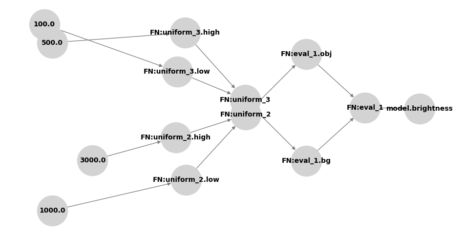
# Connected Component
dep_graph.build_subgraph("BasicMathNode:eval_1.obj", incoming=True, outgoing=True).draw()
[8]:
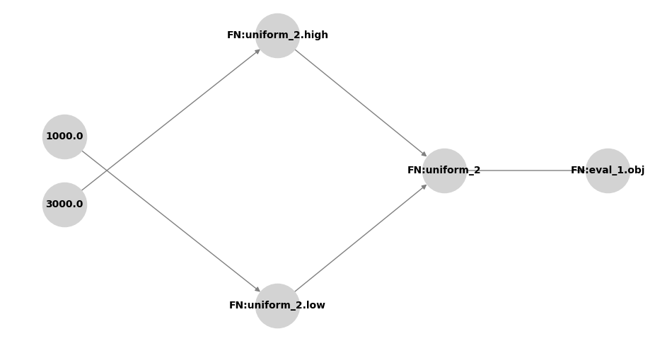
# Just parameters on which obj depends
dep_graph.build_subgraph("BasicMathNode:eval_1.obj", incoming=True, outgoing=False).draw()
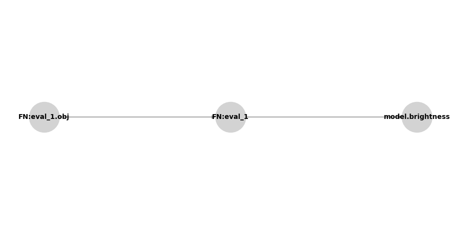
[9]:
# Just parameters that depend on obj
dep_graph.build_subgraph("BasicMathNode:eval_1.obj", incoming=False, outgoing=True).draw()