SN Ia Intrinsic Scatter Demo

This notebook demonstrates the three intrinsic scatter models available in lightcurvelynx:

• COH — coherent (gray) scatter: same magnitude offset at all wavelengths

• G10 — Guy et al. (2010) chromatic scatter derived from SALT2 color dispersion

• C11 — Chotard et al. (2011) correlated scatter across six photometric bands

We build a SALT3 simulation using SncosmoWrapperModel, attach each scatter model as a rest-frame effect via add_effect(), and measure the resulting magnitude scatter in restframe Bessell U, B, V, R, I bands.

import matplotlib.pyplot as plt
import numpy as np
import sncosmo
from lightcurvelynx.effects.snia_intrinsic_scatter import SNIaIntrinsicScatter
from lightcurvelynx.models.sncosmo_models import SncosmoWrapperModel

/home/docs/checkouts/readthedocs.org/user_builds/lightcurvelynx/envs/latest/lib/python3.12/site-packages/tqdm/auto.py:21: TqdmWarning: IProgress not found. Please update jupyter and ipywidgets. See https://ipywidgets.readthedocs.io/en/stable/user_install.html
  from .autonotebook import tqdm as notebook_tqdm

1. Build baseline SALT3 model

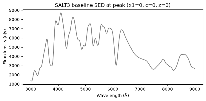
We use a canonical SN Ia at z = 0 (restframe) with parameters x₁ = 0, c = 0. The baseline SED at peak (phase = 0) is evaluated without any scatter.

# Fixed SALT3 parameters — isolates the scatter effect from parameter variation
SALT3_KWARGS = dict(t0=0.0, x0=3e-5, x1=0.0, c=0.0, redshift=0.0)

# Wavelength grid covering Bessell U–I (3000–9000 Å)
wavelengths = np.linspace(3000, 9000, 600)
times_peak = np.array([0.0])  # observer-frame MJD at peak (= t0)

baseline_model = SncosmoWrapperModel("salt3", **SALT3_KWARGS)
state = baseline_model.sample_parameters()
baseline_sed = baseline_model.evaluate_sed(times_peak, wavelengths, state)  # (1, N) nJy

fig, ax = plt.subplots(figsize=(7, 3.5))
ax.plot(wavelengths, baseline_sed[0], color="gray")
ax.set_xlabel("Wavelength (Å)")
ax.set_ylabel("Flux density (nJy)")
ax.set_title("SALT3 baseline SED at peak (x1=0, c=0, z=0)")
plt.tight_layout()

Downloading https://sncosmo.github.io/data/models/salt3/salt3-f22.tar.gz [Done]

2. Simulate scatter realizations

For each scatter model we:

1. Create a new SncosmoWrapperModel with the same fixed SALT3 parameters

2. Attach SNIaIntrinsicScatter as a rest-frame effect via add_effect()

3. Sample N states at once with model.sample_parameters(N) and iterate through them

4. Compute Δmag = −2.5 log₁₀(F_scattered / F_baseline) per band

from lightcurvelynx.astro_utils.passbands import Passband, PassbandGroup

BANDS = {"U": "bessellux", "B": "bessellb", "V": "bessellv", "R": "bessellr", "I": "besselli"}

# Build PassbandGroup from sncosmo Bessell filters
passbands = PassbandGroup(
    [
        Passband.from_sncosmo("bessell", filter_name, bandpass=bandname)
        for filter_name, bandname in BANDS.items()
    ]
)

# Baseline band fluxes via sncosmo (for display)
baseline_flux = {
    filter_name: baseline_model.source.bandflux(bandname, 0.0, zp=25.0, zpsys="ab")
    for filter_name, bandname in BANDS.items()
}
print("Baseline band fluxes (sncosmo, zp=25 AB):")
for b, f in baseline_flux.items():
    print(f"  Bessell {b}: {f:.4e}")

# Baseline integrals via evaluate_bandfluxes (for ratio)
times_bands = np.repeat(times_peak, len(BANDS))
filters_bands = np.array(list(BANDS.keys()))
baseline_arr = baseline_model.evaluate_bandfluxes(passbands, times_bands, filters_bands, state)
baseline_bandflux = {f"bessell_{f}": v for f, v in zip(BANDS.keys(), baseline_arr, strict=False)}

N = 300

SCATTER_MODELS = {
    "COH (σ=0.1)": {"modelname": "COH", "sigma": 0.1},
    "G10": {"modelname": "G10", "coh_sigma": 0.0},
    "C11": {"modelname": "C11", "coh_sigma": 0.0},
}

delta_mag = {}  # delta_mag[label][band] = (N,) array

for label, modelpars in SCATTER_MODELS.items():
    effect = SNIaIntrinsicScatter(modelpars=modelpars)
    model = SncosmoWrapperModel("salt3", **SALT3_KWARGS)
    model.add_effect(effect)  # rest_frame=True by default

    states = model.sample_parameters(num_samples=N)

    dm = {b: np.empty(N) for b in BANDS}
    for i, state_i in enumerate(states):
        band_fluxes_arr = model.evaluate_bandfluxes(passbands, times_bands, filters_bands, state_i)
        for j, filter_name in enumerate(BANDS):
            full_name = f"bessell_{filter_name}"
            dm[filter_name][i] = -2.5 * np.log10(band_fluxes_arr[j] / baseline_bandflux[full_name])
    delta_mag[label] = dm
    print(f"{label}: done")

Baseline band fluxes (sncosmo, zp=25 AB):
  Bessell U: 1.1499e+01
  Bessell B: 1.8732e+01
  Bessell V: 1.7261e+01
  Bessell R: 1.4444e+01
  Bessell I: 8.8713e+00
COH (σ=0.1): done
G10: done
C11: done

3. Magnitude scatter vs central wavelength

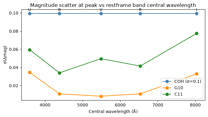
For each model, plot the rms scatter σ(Δmag) against the flux-weighted central wavelength of each Bessell band. COH (gray) should be flat; G10 and C11 should decline toward redder bands.

COLORS = {"COH (σ=0.1)": "steelblue", "G10": "darkorange", "C11": "forestgreen"}

central_wave = {
    filter_name: sncosmo.get_bandpass(bandname).wave_eff for filter_name, bandname in BANDS.items()
}
band_names = list(BANDS.keys())
x = np.array([central_wave[b] for b in band_names])

fig, ax = plt.subplots(figsize=(7, 4))
all_sigma = {}
for label, dm in delta_mag.items():
    sigma = np.array([dm[b].std() for b in band_names])
    all_sigma[label] = sigma
    ax.plot(x, sigma, "o-", color=COLORS[label], label=label, markersize=7)

# Annotate band names just above the highest σ point in each column
top_sigma = np.max(list(all_sigma.values()), axis=0)
for b, xb, yt in zip(band_names, x, top_sigma, strict=False):
    ax.annotate(b, xy=(xb, yt), xytext=(0, 6), textcoords="offset points", ha="center", fontsize=9)

ax.set_xlabel("Central wavelength (Å)")
ax.set_ylabel("σ(Δmag)")
ax.set_title("Magnitude scatter at peak vs restframe band central wavelength")
ax.legend()
plt.tight_layout()

4. Interpolation method comparison (G10 and C11)

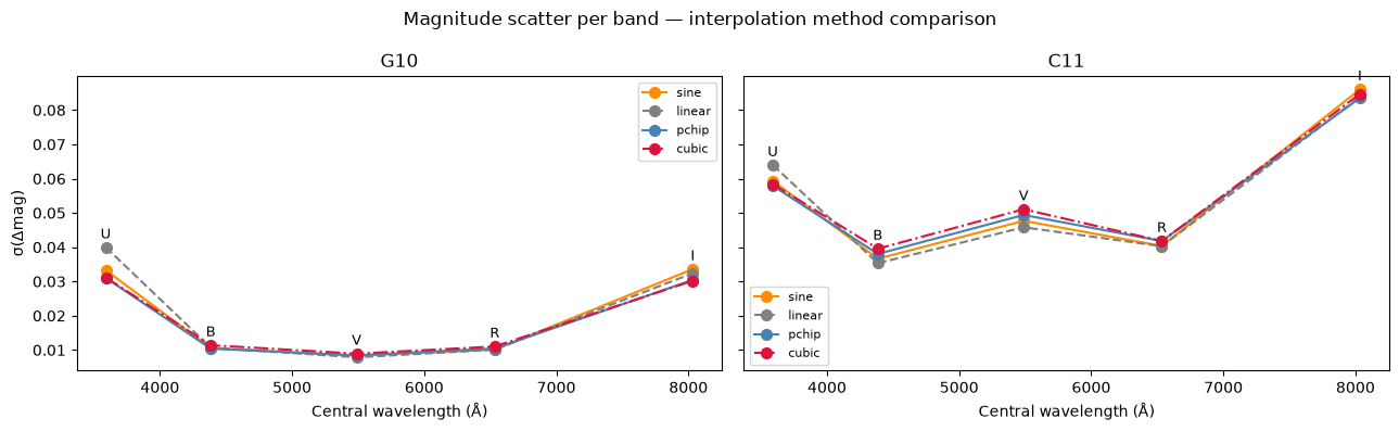
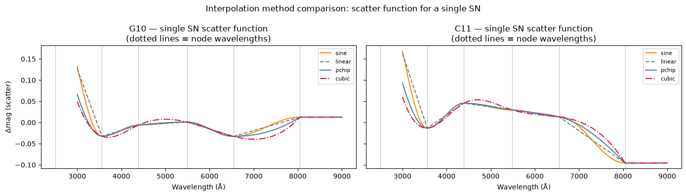
We compare four interpolation methods on the G10 model:

• sine — SNANA reference: zero derivative at each node, bounded

• linear — piecewise linear baseline

• pchip — monotone-preserving cubic Hermite: no overshoot, natural slopes at nodes

• cubic — C² cubic spline: maximally smooth, but can overshoot between nodes

First we show the scatter function λ → Δmag for a single SN realization, then the rms σ per band over N realizations.

INTERP_METHODS = ["sine", "linear", "pchip", "cubic"]
INTERP_COLORS = {"sine": "darkorange", "linear": "gray", "pchip": "steelblue", "cubic": "crimson"}
INTERP_STYLES = {"sine": "-", "linear": "--", "pchip": "-", "cubic": "-."}

g10_modelpars = {"modelname": "G10", "coh_sigma": 0.0, "sourcename": "salt3"}
c11_modelpars = {"modelname": "C11", "coh_sigma": 0.0}

# --- Single-SN scatter function ---
# Reset to the same seed for each method so node draws are identical —
# differences come purely from the interpolation shape.
fig, axes = plt.subplots(1, 2, figsize=(14, 4), sharey=True)
for ax, (label, modelpars) in zip(axes, [("G10", g10_modelpars), ("C11", c11_modelpars)], strict=False):
    for method in INTERP_METHODS:
        effect = SNIaIntrinsicScatter(modelpars=modelpars, interp_method=method)
        model = SncosmoWrapperModel("salt3", **SALT3_KWARGS)
        model.add_effect(effect)
        state_i = next(iter(model.sample_parameters(num_samples=1, rng_info=np.random.default_rng(42))))
        sed = model.evaluate_sed(times_peak, wavelengths, state_i)
        scatter_fn = -2.5 * np.log10(sed[0] / baseline_sed[0])
        ax.plot(
            wavelengths,
            scatter_fn,
            color=INTERP_COLORS[method],
            ls=INTERP_STYLES[method],
            label=method,
            lw=1.5,
        )
    for lam in [2500, 3560, 4390, 5490, 6545, 8045]:
        ax.axvline(lam, color="k", lw=0.5, ls=":")
    ax.set_xlabel("Wavelength (Å)")
    ax.set_title(f"{label} — single SN scatter function\n(dotted lines = node wavelengths)")
    ax.legend(fontsize=8)
axes[0].set_ylabel("Δmag (scatter)")
fig.suptitle("Interpolation method comparison: scatter function for a single SN")
plt.tight_layout()

# --- σ per band for each interpolation method ---
# Same seed across methods so each gets identical scatter draws —
# σ differences reflect interpolation shape only, not sampling noise.
delta_mag_interp = {}

for scatter_label, modelpars in [("G10", g10_modelpars), ("C11", c11_modelpars)]:
    delta_mag_interp[scatter_label] = {}
    for method in INTERP_METHODS:
        effect = SNIaIntrinsicScatter(modelpars=modelpars, interp_method=method)
        model = SncosmoWrapperModel("salt3", **SALT3_KWARGS)
        model.add_effect(effect)
        states = model.sample_parameters(num_samples=N, rng_info=np.random.default_rng(42))

        dm = {b: np.empty(N) for b in BANDS}
        for i, state_i in enumerate(states):
            band_fluxes_arr = model.evaluate_bandfluxes(passbands, times_bands, filters_bands, state_i)
            for j, filter_name in enumerate(BANDS):
                full_name = f"bessell_{filter_name}"
                dm[filter_name][i] = -2.5 * np.log10(band_fluxes_arr[j] / baseline_bandflux[full_name])
        delta_mag_interp[scatter_label][method] = dm

fig, axes = plt.subplots(1, 2, figsize=(13, 4), sharey=True)
for ax, scatter_label in zip(axes, ["G10", "C11"], strict=False):
    for method in INTERP_METHODS:
        sigma = np.array([delta_mag_interp[scatter_label][method][b].std() for b in band_names])
        ax.plot(
            x, sigma, "o" + INTERP_STYLES[method], color=INTERP_COLORS[method], label=method, markersize=7
        )
    top_sigma = np.max(
        [np.array([delta_mag_interp[scatter_label][m][b].std() for b in band_names]) for m in INTERP_METHODS],
        axis=0,
    )
    for b, xb, yt in zip(band_names, x, top_sigma, strict=False):
        ax.annotate(b, xy=(xb, yt), xytext=(0, 6), textcoords="offset points", ha="center", fontsize=9)
    ax.set_xlabel("Central wavelength (Å)")
    ax.set_title(f"{scatter_label}")
    ax.legend(fontsize=8)
axes[0].set_ylabel("σ(Δmag)")
fig.suptitle("Magnitude scatter per band — interpolation method comparison")
plt.tight_layout()