Using Simulated Argus Data

In this notebook we look at how we can run simulations using a simulated survey file from the Argus Array. This file uses (private) survey files that are not yet available for download.

NOTE: The ArgusHealpixObsTable is still in prototype and should not be used for scientific analysis until it is verified.

import matplotlib.pyplot as plt
import numpy as np
import pandas as pd

from lightcurvelynx import _LIGHTCURVELYNX_BASE_DATA_DIR
from lightcurvelynx.astro_utils.passbands import Passband, PassbandGroup
from lightcurvelynx.astro_utils.snia_utils import DistModFromRedshift, X0FromDistMod
from lightcurvelynx.math_nodes.np_random import NumpyRandomFunc
from lightcurvelynx.math_nodes.ra_dec_sampler import ApproximateMOCSampler
from lightcurvelynx.models.sncosmo_models import SncosmoWrapperModel
from lightcurvelynx.obstable.argus_obstable import ArgusHealpixObsTable
from lightcurvelynx.simulate import simulate_lightcurves
from lightcurvelynx.survey_info import SurveyInfo
from lightcurvelynx.utils.extrapolate import ZeroPadding
from lightcurvelynx.utils.plotting import plot_lightcurves

Argus Survey Data

We start by loading an simulated argus survey file. Unlike the other survey tables, Argus stores information indexed by healpix. Each entry contains the information for a single healpix and time (epoch). The example file we use (“argussim_hpx_6131.parquet”) includes information for a single healpix tile.

table = pd.read_parquet(_LIGHTCURVELYNX_BASE_DATA_DIR / "opsim" / "argussim_hpx_6131.parquet")
print(f"Loaded table with {len(table)} rows and columns: {table.columns.tolist()}")
table.head()

Loaded table with 2379615 rows and columns: ['ra', 'dec', 'alt', 'az', 'nside', 'masked', 'epoch', 'exptime', 'ratchnum', 'seeing', 'moon_alt', 'moon_frac', 'limmag', 'sky_brightness', 'distance', 'volume', 'nested', 'signal_electrons', 'readnoise', 'dark_electrons', 'sky_electrons', 'noise', 'sharpness']

	ra	dec	alt	az	nside	masked	epoch	exptime	ratchnum	seeing	...	sky_brightness	distance	volume	nested	signal_electrons	readnoise	dark_electrons	sky_electrons	noise	sharpness
healpix
6131	89.83966	34.272703	85.944664	333.864238	32	False	52222.409375	60.0	35	0.804956	...	21.426368	179.419602	4.703139e+06	1	210.638797	2.980317	0.405696	243.357877	21.524048	0.325367
6131	89.83966	34.272703	85.944664	333.864238	32	False	52222.410069	60.0	35	0.804956	...	21.426368	179.419602	4.703139e+06	1	210.638797	2.980317	0.405696	243.357877	21.524048	0.325367
6131	89.83966	34.272703	85.944664	333.864238	32	False	52222.410764	60.0	35	0.804956	...	21.426368	179.419602	4.703139e+06	1	210.638797	2.980317	0.405696	243.357877	21.524048	0.325367
6131	89.83966	34.272703	85.944664	333.864238	32	False	52222.411458	60.0	35	0.804956	...	21.426368	179.419602	4.703139e+06	1	210.638797	2.980317	0.405696	243.357877	21.524048	0.325367
6131	89.83966	34.272703	85.944664	333.864238	32	False	52222.412153	60.0	35	0.804956	...	21.426368	179.419602	4.703139e+06	1	210.638797	2.980317	0.405696	243.357877	21.524048	0.325367

5 rows × 23 columns

We can use the ArgusHealpixObsTable class to transform the simulated data into an ObsTable data structure that can be used with LightCurveLynx’s simulation infrastructure. This class performs several important preprocessing steps including: 1) Mapping the column names to standard names, 2) deriving noise information (zero points), and 3) building spatial data structures for fast querying.

Currently there are a few restrictions in the ArgusHealpixObsTable class that can be relaxed if needed. Primarily all entries are required to use the same healpix order (nside).

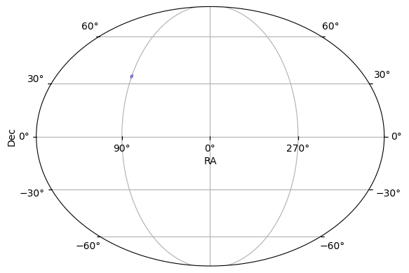
After loading the table, we plot the footprint on the sky.

ops_data = ArgusHealpixObsTable(table)
print(f"ObsTable has {len(ops_data)} rows and columns: {ops_data.columns.tolist()}")
ops_data.plot_footprint()

ObsTable has 2379615 rows and columns: ['healpix', 'ra', 'dec', 'alt', 'az', 'nside', 'masked', 'time', 'exptime', 'ratchnum', 'seeing', 'moon_alt', 'moon_frac', 'maglim', 'skybrightness', 'distance', 'volume', 'nested', 'signal_electrons', 'readnoise', 'dark_electrons', 'sky_bg_e', 'noise', 'sharpness', 'filter', 'dark_current', 'zp', 'psf_footprint']

(<Figure size 640x480 with 1 Axes>, <WCSAxes: >)

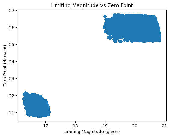
We derive a zero point from a variety of factors including the limiting magnitude, exposure time, seeing, data electrons, and sky electrons. This is currently an approximation and we will need to work with the Argus team to best capture how to survey characteristics.

We can see two distinct clusters corresponding to the 60s and 1s exposures.

plt.scatter(
    ops_data["maglim"].to_numpy(),
    ops_data["zp"].to_numpy(),
    alpha=0.5,
)
plt.xlabel("Limiting Magnitude (given)")
plt.ylabel("Zero Point (derived)")
plt.title("Limiting Magnitude vs Zero Point")
plt.show()

By the survey’s nature the Argus data has a huge number of observations.

t_min, t_max = ops_data.time_bounds()
print(f"Found {len(ops_data)} observations in time range [{t_min}, {t_max}]")

Found 2379615 observations in time range [51544.0875, 53370.44097222222]

For the purposes of this notebook, we are going to just use 90 days worth of data. The filter_rows() handles updating the observation table so as to keep all the metadata current.

t_max = t_min + 90
time_mask = ops_data["time"] <= t_max
ops_data.filter_rows(time_mask)

print(f"After filtering to 90 days, {len(ops_data)} observations remain in time range [{t_min}, {t_max}]")

After filtering to 90 days, 149235 observations remain in time range [51544.0875, 51634.0875]

Filter Information

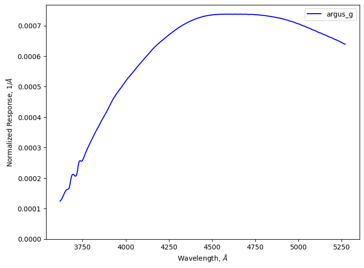
The second piece of survey information that we need to run the simulation is the filter information. For this notebook, we will use custom ‘g’ filter provided by the argus team.

Note that for efficiency, the Passband class will automatically trim the transmission curve to only keep the central 99.8% of the data. So, while the file specifies wavelengths from 3,000 A to 10,000 A, the stored data will only cover the range of 3,620 A to 5,270 A. This setting can be adjusted using the trim_quantile argument, such as setting it to 1e-8 to get almost the full range.

# Load the g-band passband for Argus from a given file.
g_passband = Passband.from_file(
    "argus",  # survey name
    "g",  # filter name
    table_path=_LIGHTCURVELYNX_BASE_DATA_DIR / "passbands" / "argus_g_wav.parquet",
    units="nm",
)
print(f"Loaded g-band passband with wave range {g_passband.waves[0]}-{g_passband.waves[-1]} Angstroms.")

# Create a PassbandGroup with only the g-band and plot it.
pb_group = PassbandGroup([g_passband])
pb_group.plot()

Loaded g-band passband with wave range 3620.0-5270.0 Angstroms.

The combination of the observations table and the bandpass filter provide all the survey information we need for the simulation. Next up is the model itself.

Create the model

To generate simulated light curves we need to define the properties of the object from which to sample. In this notebook, we use sncosmo’s SALT2 model for Type Ia supernova.

We start with “sampler” nodes that specify the distribution from which we would like to sample the object’s parameters. We use the survey data to generate a multi-order coverage map of the survey footprint and sample (RA, dec) from that footprint. We sample redshift uniformly from [0.001, 0.2].

ra_dec_sampler = ApproximateMOCSampler.from_obstable(ops_data, depth=ops_data.healpix_depth)
redshift_sampler = NumpyRandomFunc("uniform", low=0.01, high=0.2)

We compute the physical parameters as follows:

# Use given values the cosmological parameters (H0=73.0, Omega_m=0.3).
# Then compue the distance modulus from the redshift (taking the redshift sampler as input).
distmod_func = DistModFromRedshift(redshift_sampler, H0=73.0, Omega_m=0.3)

# Sample x1, c, and m_abs from distributions motivated by typical SNIa values.
x1_func = NumpyRandomFunc("normal", loc=0, scale=2.0)
c_func = NumpyRandomFunc("normal", loc=0, scale=0.02)
m_abs_func = NumpyRandomFunc("normal", loc=-19.3, scale=0.1)

# Compute x0 from the other parameters using the standard Tripp formula,
# and the distance modulus from above.
x0_func = X0FromDistMod(
    distmod=distmod_func,  # Use the computed distance modulus from redshift as input.
    x1=x1_func,  # Use the sampled x1 values as input.
    c=c_func,  # Use the sampled c values as input.
    alpha=0.14,  # Use a constant alpha value motivated by typical SNIa fits.
    beta=3.1,  # Use a constant beta value motivated by typical SNIa fits.
    m_abs=m_abs_func,  # Use the sampled m_abs values as input.
)

# t0 for the super nova is sampled uniformly over the time range of the observations.
t0_func = NumpyRandomFunc("uniform", low=t_min, high=t_max)

Note that for more realistic surveys, we would likely want to first sample the host galaxy’s properties (using something like pzflow to define its parameters) and then sample the SALT2 parameters based on the host’s details. In general, LightCurveLynx provides the ability to define a complex directed acyclic graph (DAG) of parameters.

We then define the model using the SncosmoWrapperModel class. All of the parameters are set using the samplers defined above.

source = SncosmoWrapperModel(
    "salt2-h17",  # Model name
    t0=t0_func,
    x0=x0_func,
    x1=x1_func,
    c=c_func,
    ra=ra_dec_sampler.ra,
    dec=ra_dec_sampler.dec,
    redshift=redshift_sampler,
    node_label="source",
    time_extrapolation=ZeroPadding(),
)

Generate the simulations

We can now generate random simulations with all the information defined above. The light curves are written in the nested-pandas format for easy analysis.

Note: This cell will take multiple minutes to run. We don’t show the progress bars, because they do not work well with parallel runs.

lightcurves = simulate_lightcurves(
    source,  # The model we are simulating.
    20,  # The number of simulations to run,
    SurveyInfo(obstable=ops_data, passbands=pb_group),  # The survey info
    num_jobs=8,  # Use 8 workers to speed up the simulation.
    progress_bar=False,  # Do not show the progress bar (since we are only running in parallel)
)

# Drop the parameters column to make the output more concise.
lightcurves = lightcurves.drop(columns=["params"])
lightcurves.head()

/Users/jkubica/h/lightcurvelynx/src/lightcurvelynx/noise_models/noise_utils.py:81: RuntimeWarning: invalid value encountered in sqrt
  return np.sqrt(total_variance) * zp

	id	ra	dec	nobs	t0	z	lightcurve
0	0	89.817732	34.349335	149235	51617.346507	0.022544	mjd filter ... obs_idx is_saturated 51587.26875 g ... 0 False +149234 rows ... ... ... ...
1	1	90.278975	35.206632	149235	51632.833578	0.134351	mjd filter ... obs_idx is_saturated 51587.26875 g ... 0 False +149234 rows ... ... ... ...
2	2	89.898150	32.932843	149235	51571.066117	0.145702	mjd filter ... obs_idx is_saturated 51587.26875 g ... 0 False +149234 rows ... ... ... ...
3	3	90.035246	34.776475	149235	51597.914857	0.132374	mjd filter ... obs_idx is_saturated 51587.26875 g ... 0 False +149234 rows ... ... ... ...
4	4	91.208162	34.395231	149235	51570.876276	0.060921	mjd filter ... obs_idx is_saturated 51587.26875 g ... 0 False +149234 rows ... ... ... ...

5 rows x 7 columns

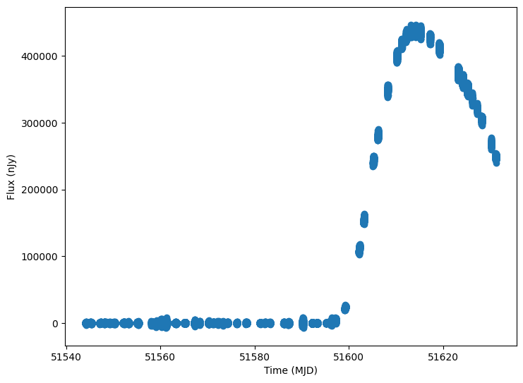
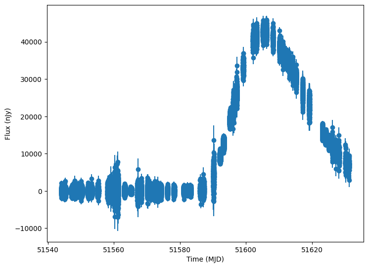
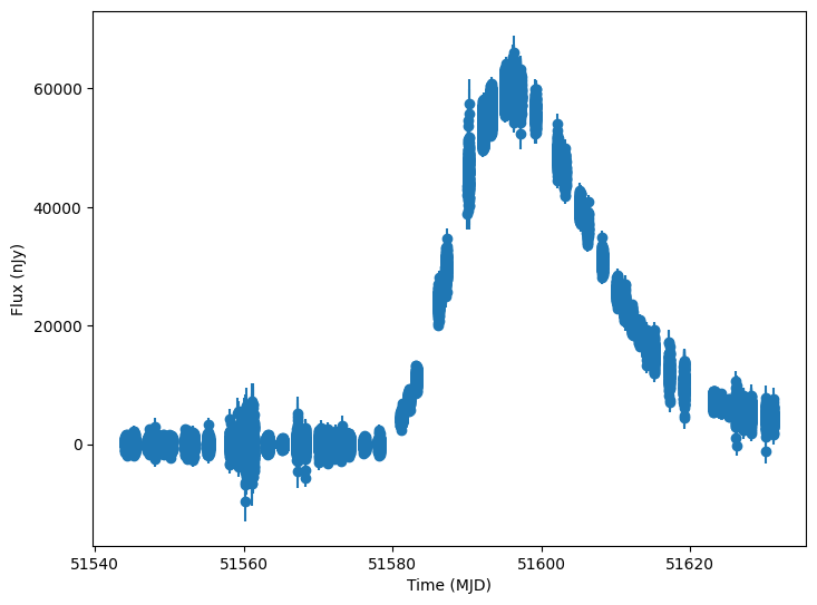
Now let’s plot some random light curves

lightcurves = lightcurves.dropna(subset=["lightcurve"])
random_ids = np.random.choice(len(lightcurves), 3)

for random_id in random_ids:
    # Extract the row for this object.
    lc = lightcurves.iloc[random_id]

    # Unpack the nested columns (filters, mjd, flux, and flux error).
    lc_filters = np.asarray(lc["lightcurve"]["filter"], dtype=str)
    lc_mjd = np.asarray(lc["lightcurve"]["mjd"], dtype=float)
    lc_flux = np.asarray(lc["lightcurve"]["flux"], dtype=float)
    lc_fluxerr = np.asarray(lc["lightcurve"]["fluxerr"], dtype=float)

    plot_lightcurves(
        fluxes=lc_flux,
        times=lc_mjd,
        fluxerrs=lc_fluxerr,
        filters=lc_filters,
    )