Simulations using the LocationFreeObsTable

In this notebook we look at how we can run simulations using an LocationFreeObsTable, which does not do any filtering on position. This ObsTable type is provided to enable comparison with actual survey cadences or to test “ideal” cadences.

To generate a simulation, we need a few pieces of information:

• The table of observations (LocationFreeObsTable)

• The filter information - We will use the LSST filters

• The noise model - We will use Gaussian noise with a constant standard deviation.

• The object model - We use a SALT2 model of SNIa

We create each one below.

Creating Survey Information

The first three pieces of data (table of observations, filter information, and noise model) are part of the survey information.

LocationFreeObsTable

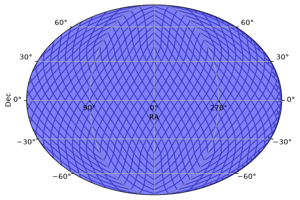
Unlike the other ObsTable types, the LocationFreeObsTable requires only two columns “time” and “filter”. We start with a simple table that has one observation per day in each “g” and “r” filters. By definition of the LocationFreeObsTable, its footprint covers the entire sky.

import numpy as np

from lightcurvelynx.obstable.location_free_obstable import LocationFreeObsTable

mjd_times = np.array([59580.0, 59580.1, 59581.0, 59581.1, 59582.0, 59582.1, 59590.0, 59590.1])
filters = np.array(["g", "r", "g", "r", "g", "r", "g", "r"])
data = {"time": mjd_times, "filter": filters}

obs_table = LocationFreeObsTable(data)
obs_table.plot_footprint(depth=5)

(<Figure size 640x480 with 1 Axes>, <WCSAxes: >)

Filter Information

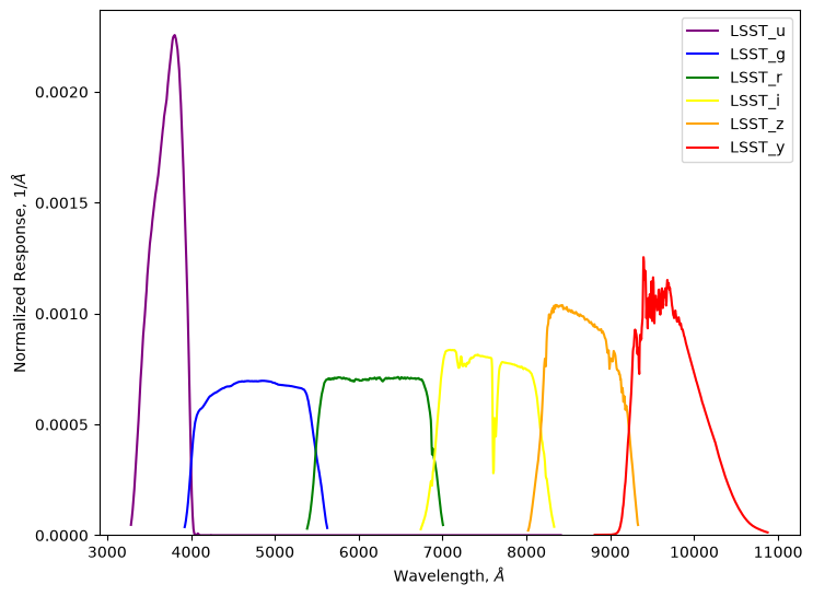
The second piece of survey information that we need to run the simulation is the filter information. By default LocationFreeObsTable does not have predefined filters. We will want to use the same filters from the survey we are using for comparison. Let’s test with LSST’s filter set.

from lightcurvelynx.astro_utils.passbands import PassbandGroup

pb_group = PassbandGroup.from_preset(preset="LSST")
pb_group.plot()

/home/docs/checkouts/readthedocs.org/user_builds/lightcurvelynx/envs/stable/lib/python3.12/site-packages/tqdm/auto.py:21: TqdmWarning: IProgress not found. Please update jupyter and ipywidgets. See https://ipywidgets.readthedocs.io/en/stable/user_install.html
  from .autonotebook import tqdm as notebook_tqdm

Downloading data file from https://raw.githubusercontent.com/lsst/throughputs/main/baseline/total_u.dat to /home/docs/.cache/lightcurvelynx/passbands/LSST/u.dat
Downloading data file from https://raw.githubusercontent.com/lsst/throughputs/main/baseline/total_g.dat to /home/docs/.cache/lightcurvelynx/passbands/LSST/g.dat
Downloading data file from https://raw.githubusercontent.com/lsst/throughputs/main/baseline/total_r.dat to /home/docs/.cache/lightcurvelynx/passbands/LSST/r.dat
Downloading data file from https://raw.githubusercontent.com/lsst/throughputs/main/baseline/total_i.dat to /home/docs/.cache/lightcurvelynx/passbands/LSST/i.dat
Downloading data file from https://raw.githubusercontent.com/lsst/throughputs/main/baseline/total_z.dat to /home/docs/.cache/lightcurvelynx/passbands/LSST/z.dat
Downloading data file from https://raw.githubusercontent.com/lsst/throughputs/main/baseline/total_y.dat to /home/docs/.cache/lightcurvelynx/passbands/LSST/y.dat

Noise Model

The final piece of survey information that we need is a noise model. In this example, we use Gaussian noise with a constant standard deviation (5.0 nJy).

from lightcurvelynx.noise_models.base_noise_models import ConstantFluxNoiseModel

noise_model = ConstantFluxNoiseModel(5.0)

Users can select more realistic noise models as long as the necessary information is available in the ObsTable. See the documentation about noise models for more details.

Given this information we can create a SurveyInfo object that wraps everything we want to simulate about the survey.

from lightcurvelynx.survey_info import SurveyInfo

survey_info = SurveyInfo(
    obstable=obs_table,
    passbands=pb_group,
    noise_model=noise_model,
    survey_name="test_survey",
)

Creating the Supernova Model

To generate simulated light curves we need to define the properties of the object from which to sample. In this notebook, we use sncosmo’s SALT2 model for Type Ia supernova.

We start with “sampler” nodes that specify the distribution from which we would like to sample the object’s parameters. Since we are not filtering on position, we will use ra=0.0 and dec=0.0. We sample redshift uniformly from [0.001, 0.1].

from lightcurvelynx.math_nodes.np_random import NumpyRandomFunc

redshift_sampler = NumpyRandomFunc("uniform", low=0.001, high=0.1)

We compute the physical parameters as follows:

from lightcurvelynx.astro_utils.snia_utils import DistModFromRedshift, X0FromDistMod

# Use the given values for the cosmological parameters (H0=73.0, Omega_m=0.3).
# Then compute the distance modulus from the redshift (taking the redshift sampler as input).
distmod_func = DistModFromRedshift(redshift_sampler, H0=73.0, Omega_m=0.3)

# Sample x1, c, and m_abs from distributions motivated by typical SNIa values.
x1_func = NumpyRandomFunc("normal", loc=0, scale=2.0)
c_func = NumpyRandomFunc("normal", loc=0, scale=0.02)
m_abs_func = NumpyRandomFunc("normal", loc=-19.3, scale=0.1)

# Compute x0 from the other parameters using the standard Tripp formula,
# and the distance modulus from above.
x0_func = X0FromDistMod(
    distmod=distmod_func,  # Use the computed distance modulus from redshift as input.
    x1=x1_func,  # Use the sampled x1 values as input.
    c=c_func,  # Use the sampled c values as input.
    alpha=0.14,  # Use a constant alpha value motivated by typical SNIa fits.
    beta=3.1,  # Use a constant beta value motivated by typical SNIa fits.
    m_abs=m_abs_func,  # Use the sampled m_abs values as input.
)

# t0 for the supernova is sampled uniformly over the time range of the observations.
t0_func = NumpyRandomFunc("uniform", low=np.min(obs_table["time"]), high=np.max(obs_table["time"]))

Note that for more realistic surveys, we would likely want to first sample the host galaxy’s properties (using something like pzflow to define its parameters) and then sample the SALT2 parameters based on the host’s details. In general, LightCurveLynx provides the ability to define a complex directed acyclic graph (DAG) of parameters.

We then define the model using the SncosmoWrapperModel class. All of the parameters are set using the samplers defined above. We add linear extrapolation for times defined outside the sncosmo model’s bounds.

from lightcurvelynx.models.sncosmo_models import SncosmoWrapperModel
from lightcurvelynx.utils.extrapolate import LinearDecay

source = SncosmoWrapperModel(
    "salt2-h17",  # Model name
    t0=t0_func,
    x0=x0_func,
    x1=x1_func,
    c=c_func,
    ra=0.0,  # Use a fixed RA value for the source.
    dec=0.0,  # Use a fixed Dec value for the source.
    redshift=redshift_sampler,
    node_label="source",
    time_extrapolation=LinearDecay(50.0),
)

Downloading https://sncosmo.github.io/data/models/snana/salt2-h17.tar.gz [Done]

Generating the simulations

We can now generate random simulations with all the information defined above. The light curves are written in the nested-pandas format for easy analysis.

from lightcurvelynx.simulate import simulate_lightcurves

lightcurves = simulate_lightcurves(
    source,  # The model we are simulating.
    100,  # The number of simulations to run,
    survey_info,  # The survey information
)

# Show the first few entries (dropping the params column for display purposes).
lightcurves.drop(columns=["params"]).head()

Simulating: 100%|██████████| 100/100 [00:00<00:00, 1330.19obj/s]

	id	ra	dec	nobs	t0	z	lightcurve
0	0	0.000000	0.000000	8	59581.523323	0.012321	mjd filter ... obs_idx is_saturated 59580.0 g ... 0 False +7 rows ... ... ... ...
1	1	0.000000	0.000000	8	59583.474854	0.043246	mjd filter ... obs_idx is_saturated 59580.0 g ... 0 False +7 rows ... ... ... ...
2	2	0.000000	0.000000	8	59587.837937	0.008753	mjd filter ... obs_idx is_saturated 59580.0 g ... 0 False +7 rows ... ... ... ...
3	3	0.000000	0.000000	8	59581.551193	0.086306	mjd filter ... obs_idx is_saturated 59580.0 g ... 0 False +7 rows ... ... ... ...
4	4	0.000000	0.000000	8	59589.241991	0.009521	mjd filter ... obs_idx is_saturated 59580.0 g ... 0 False +7 rows ... ... ... ...

5 rows x 7 columns

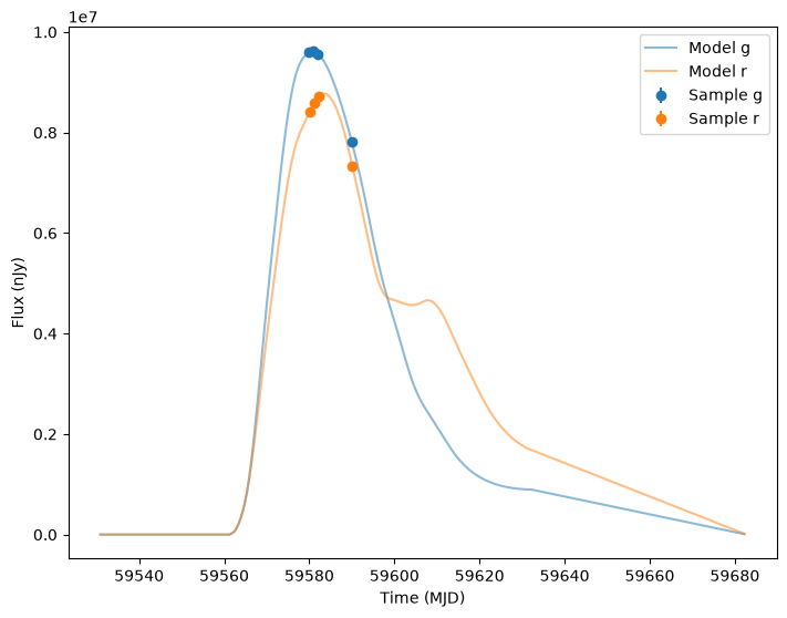
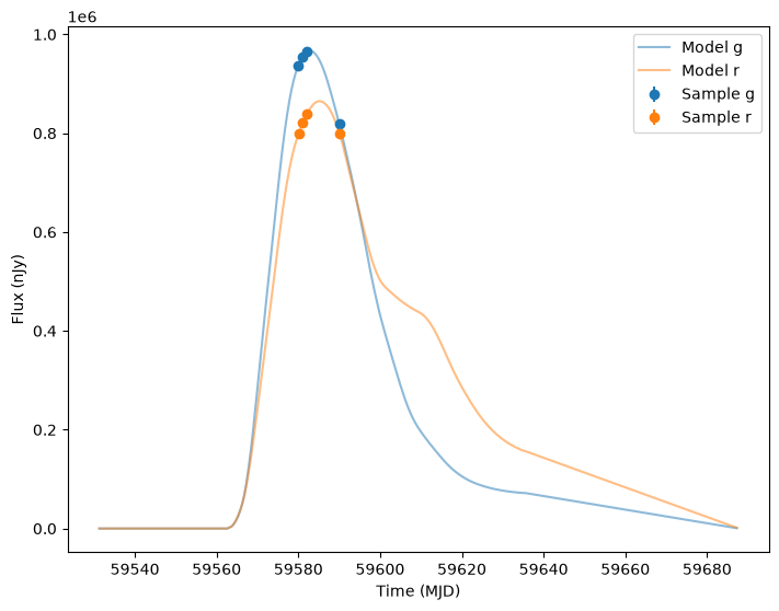
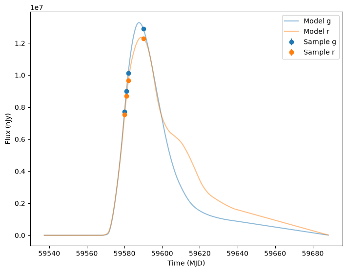
Now let’s plot the first three random light curves. For reference we will also plot the underlying curve.

from lightcurvelynx.simulate import compute_single_noise_free_lightcurve
from lightcurvelynx.graph_state import GraphState
from lightcurvelynx.utils.plotting import plot_lightcurves

for idx in range(3):
    # Extract the row for this object.
    lc = lightcurves.iloc[idx]

    # Unpack the nested columns (filters, mjd, flux, and flux error). This is the
    # data from the simulation itself.
    lc_filters = np.asarray(lc["lightcurve"]["filter"], dtype=str)
    lc_mjd = np.asarray(lc["lightcurve"]["mjd"], dtype=float)
    lc_flux = np.asarray(lc["lightcurve"]["flux"], dtype=float)
    lc_fluxerr = np.asarray(lc["lightcurve"]["fluxerr"], dtype=float)

    # Extract the parameters used during the simulation of this object (stored in the "params" column).
    # Use that to compute the noise-free light curve for this object, which we will plot alongside the
    # simulated light curve.
    noise_free_lcs = compute_single_noise_free_lightcurve(
        source,
        GraphState.from_dict(lc["params"]),
        pb_group,
        rest_frame_phase_min=-50.0,  # 50 days before t0
        rest_frame_phase_max=100.0,  # 100 days after t0
        rest_frame_phase_step=0.5,  # 2 samples per day
    )

    plot_lightcurves(
        fluxes=lc_flux,
        times=lc_mjd,
        fluxerrs=lc_fluxerr,
        filters=lc_filters,
        underlying_model=noise_free_lcs,
    )