Redback Example

In this notebook we look at how we can import and use models from the redback package, a package for transient modeling and fitting.

Note that the bilby and redback packages are not installed as part of the default LightCurveLynx installation. Users will need to manually install them via pip (e.g. pip install bilby redback) in order to run this notebook.

import numpy as np
import matplotlib.pyplot as plt

from redback import model_library
from redback.priors import get_priors

from lightcurvelynx.astro_utils.passbands import PassbandGroup
from lightcurvelynx.math_nodes.np_random import NumpyRandomFunc
from lightcurvelynx.math_nodes.ra_dec_sampler import ObsTableRADECSampler
from lightcurvelynx.obstable.opsim import OpSim
from lightcurvelynx.simulate import simulate_lightcurves
from lightcurvelynx.survey_info import SurveyInfo
from lightcurvelynx.models.redback_models import RedbackWrapperModel
from lightcurvelynx.utils.extrapolate import ConstantPadding
from lightcurvelynx.utils.plotting import plot_lightcurves

from lightcurvelynx import _LIGHTCURVELYNX_BASE_DATA_DIR

# Reset the matplotlib configuration
plt.rcParams.update(plt.rcParamsDefault)

# Set the seed so we don't get different results each time we run the notebook.
np.random.seed(42)

No module named 'lalsimulation'
lalsimulation is not installed. Some EOS based models will not work. Please use bilby eos or pass your own EOS generation class to the model
swifttools not available. You will not be able to download Swift afterglow data via API.
10:00 bilby INFO    : Running bilby version: 2.8.0
10:00 redback INFO    : Running redback version: 1.16.0

Load Data Files

We start by loading the files we will need for running the simulation: the OpSim database and the passband information. Both of these live in the data/ directory in the root directory. Note that nothing in this directory is saved to github, so the files might have to be downloaded initially.

We are getting Rubin OpSim data from the OpSim database.

We only care about the observations in the OpSim in the filters we wish to simulate. So we use OpSim.filter_rows() to remove those rows that do not match.

# Choose which filters to simulate.
filters = ["g", "r", "i", "z"]

# Load the OpSim data.
opsim_db = OpSim.from_url(
    "https://s3df.slac.stanford.edu/data/rubin/sim-data/sims_featureScheduler_runs5.3/baseline/baseline_v5.3.0_10yrs.db"
)
print(f"Loaded OpSim with {len(opsim_db)} rows.")

# Filter to only the rows that match the filters we want to simulate.
filter_mask = np.isin(opsim_db["filter"], filters)
opsim_db = opsim_db.filter_rows(filter_mask)

# Print the number of rows and time bounds after filtering.
t_min, t_max = opsim_db.time_bounds()
print(f"Filtered OpSim to {len(opsim_db)} rows and times [{t_min}, {t_max}]")

# Load the passband data for the griz filters only.
table_dir = _LIGHTCURVELYNX_BASE_DATA_DIR / "passbands" / "LSST"
passband_group = PassbandGroup.from_preset(
    preset="LSST",
    filters=filters,
    units="nm",
    trim_quantile=0.001,
    delta_wave=1,
    table_dir=table_dir,
)

survey_info = SurveyInfo(obstable=opsim_db, passbands=passband_group)

Loaded OpSim with 1844571 rows.
Filtered OpSim to 1421879 rows and times [61208.42731204634, 64860.44487408427]

Create the model

We want to create a model that uses the predefined redback model from its library. Redback offers an extensive collection of models that can be accessed by name. For a list see here. For this example, we choose the “one_component_kilonova_model” model. We look up the model using the redback.model_library.all_models_dict dictionary.

Note that redback models are defined as functions. All parameters, such as redshift or ejecta mass, are passed into this function as keyword arguments. As we will see shortly, LightCurveLynx handles the conversion of sampled parameters into keyword parameters behind the scenes.

rb_model = model_library.all_models_dict["one_component_kilonova_model"]

Next we create a wrapper RedbackWrapperModel which brings the redback model into the LightCurveLynx API space. This wrapper handles everything from the interpretation of parameters to the conversion of units (redback and LightCurveLynx use different default units). It requires three pieces of information: the model function (or name), the model’s parameters, and the model’s phase bounds.

As in other examples, we want to make the parameters dynamic to mirror a real simulation. Let’s start by drawing:

• The location (RA, dec, both in degrees) uniformly from the footprint of the survey.

• The start time (t0, days) uniformly from the coverage of the survey.

• The redshift uniformly from [0.0, 0.1]

• The mass ejecta (mej, solar masses) as a Gaussian with mean 0.05

For the rest of the parameters we will set as constants (though these could also use samplers):

• Gray opacity (kappa, cm^2/g) = 1

• Temperature floor in K (temperature_floor, kelvins) = 3000

• Minimum initial velocity (vej, fraction of the speed of light) = 0.2

Note: Unlike the other PhysicalModel classes, we will not pass all parameters as keyword arguments. The RedbackWrapperModel constructor takes a dictionary of parameters needed for that model. The dictionary maps parameter name to its setter.

Later in this notebook, we will see how we can instead use predfined redback priors to take advantage of their excellent library.

# Use an OpSim based sampler for position.
ra_dec_sampler = ObsTableRADECSampler(
    opsim_db,
    radius=3.0,  # degrees
    node_label="ra_dec_sampler",
)

# Use a uniform sampler for the starting time (t0) of activity.
time_sampler = NumpyRandomFunc("uniform", low=t_min, high=t_max, node_label="time_sampler")

# Set the parameters that are needed by the redback model. Note that the first two are set
# from samplers, while the last three are fixed values.
parameters = {
    "mej": NumpyRandomFunc("normal", loc=0.05, scale=0.02),
    "redshift": NumpyRandomFunc("uniform", low=0.0, high=0.1),
    "temperature_floor": 3000,
    "kappa": 1,
    "vej": 0.2,
}

# Create the model itself.
source = RedbackWrapperModel(
    rb_model,
    parameters=parameters,  # Set ALL the redback model parameters
    ra=ra_dec_sampler.ra,  # Set other parameters
    dec=ra_dec_sampler.dec,
    t0=time_sampler,
    node_label="source",
    phase_bounds=(0.1, 50.0),  # The kilonova model is only valid in this phase range, so we set it here
    time_extrapolation=(ConstantPadding(0.0), ConstantPadding(0.0)),
)

Here we set the phase bounds based on our knowledge of redback’s kilonova model. But the phase bounds will vary with different types of models and simulation goals. For most redback’s explosion-based models, the valid phase_bound range would be (1.e-3, None), indicating 0.001 < t0 < inf.

Users should consult with the redback documentation or team for valid phase_bound values.

Generate the simulations

We can now generate random simulations with all the information defined above. The simulate_lightcurves function takes four parameters: the source from which we want to sample (here the collection of lightcurves), the number of results to simulate (100), the opsim, and the passband information.

Since Redback’s the one component kilanova model is only defined after time t0, we use the rest_time_window_offset parameter to limit the samples for each object to 0 days before and 50 days after that object’s t0. These bounds are provided in the rest frame.

lightcurves = simulate_lightcurves(
    source,
    100,
    survey_info,
    rest_time_window_offset=(-100.0, 100),  # one_component_kilonova_model only works for t > 0
)

Simulating: 100%|██████████| 100/100 [00:02<00:00, 45.97obj/s]

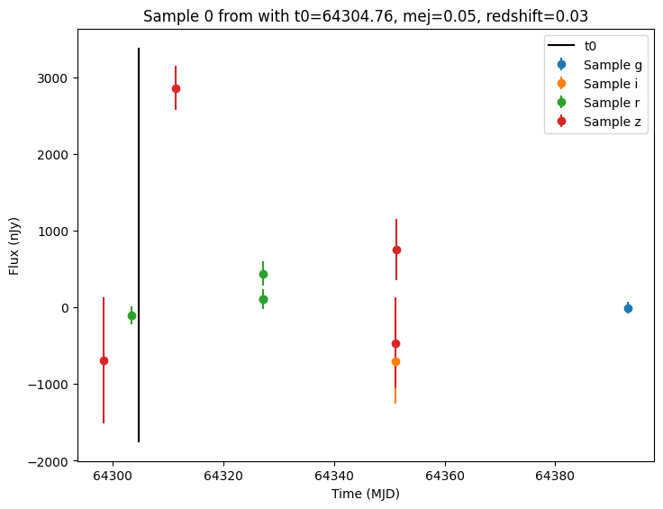
The results are written in the nested-pandas format for easy analysis. Each row corresponds to a single simulated object, with a unique id, ra, dec, etc. The column params include all internal state, including hyperparameter settings, that was used to generate this object. The nested lightcurve column contains the times, filters, and fluxes for each observation of that object. We can treat it as a (nested) table.

Let’s look at the lightcurve for the first object sampled:

print(lightcurves.loc[0]["lightcurve"])

            mjd filter         flux     fluxerr  flux_perfect  survey_idx  \
0  64298.349999      z  -690.463102  823.876707      0.000000           0
1  64303.314912      r  -103.885617  115.442839      0.000000           0
2  64311.332008      z  2860.190232  284.389363   2792.549403           0
3  64327.101776      g   106.571144   84.205290     14.443455           0
4  64327.125533      r   104.479438  127.876003     63.477938           0
5  64327.202313      r   440.075495  162.404540     63.092202           0
6  64351.065303      i  -698.431822  552.780464     41.134880           0
7  64351.088857      z  -462.984323  595.586636     95.214257           0
8  64351.298833      z   751.866209  398.966547     95.030516           0
9  64393.115399      g    -7.627442   77.689849      0.000000           0

   obs_idx  is_saturated
0  1174983         False
1  1177499         False
2  1179924         False
3  1186909         False
4  1186961         False
5  1187118         False
6  1195560         False
7  1195612         False
8  1196080         False
9  1218586         False

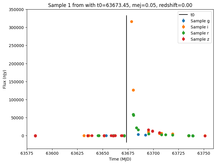
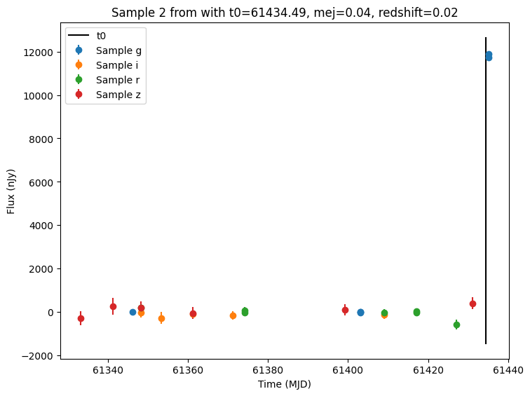
Now let’s plot the first few lightcurves to see what they look like when observed via Rubin’s cadence.

for idx in range(3):
    # Extract the row for this object.
    lc = lightcurves.loc[idx]

    if lc["nobs"] == 0:
        continue

    # Unpack the nested columns (filters, mjd, flux, and flux error).
    lc_filters = np.asarray(lc["lightcurve"]["filter"], dtype=str)
    lc_mjd = np.asarray(lc["lightcurve"]["mjd"], dtype=float)
    lc_flux = np.asarray(lc["lightcurve"]["flux"], dtype=float)
    lc_fluxerr = np.asarray(lc["lightcurve"]["fluxerr"], dtype=float)

    # Get information about the sampled parameter values for the plot's title.
    t0 = lc["params"]["source.t0"]
    mej = lc["params"]["source.mej"]
    redshift = lc["params"]["source.redshift"]

    zoom_inds = (lc_mjd > t0 - 500) & (lc_mjd < t0 + 2000)

    # Plot the lightcurves.
    ax = plot_lightcurves(
        fluxes=lc_flux[zoom_inds],
        times=lc_mjd[zoom_inds],
        fluxerrs=lc_fluxerr[zoom_inds],
        filters=lc_filters[zoom_inds],
        title=f"Sample {idx} from with t0={t0:.2f}, mej={mej:.2f}, redshift={redshift:.2f}",
    )
    ax.plot([t0, t0], ax.get_ylim(), "k-", label="t0")
    ax.legend()
    plt.show()

Zooming In

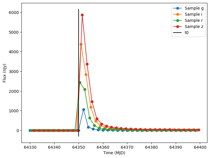
As you can see from the plots above, the combination of a random sampling scheme for t0 combined with the Rubin OpSim, might mean that we miss the kilanova event in the data. While this is exactly the type of behavior we want to be able to characterize for analyzing the survey’s selection function, we might want to see what the event looks like under ideal conditions.

Let’s zoom in, by creating a fixed kilanova object and a custom observing strategy. We will use evaluate_bandfluxes to compute the noise free bandfluxes at a set of times (instead of matching the times with the observation table).

# Set fixed parameters for this redback model.
t0 = 64350.0
parameters = {
    "mej": 0.05,
    "redshift": 0.05,
    "temperature_floor": 3000,
    "kappa": 1,
    "vej": 0.2,
}
source = RedbackWrapperModel(
    rb_model,
    parameters=parameters,  # Set ALL the redback model parameters
    ra=0.0,  # Set other parameters
    dec=-10.0,
    t0=t0,
    phase_bounds=(0.1, 50.0),  # The kilonova model is only valid in this phase range
    node_label="source",
    time_extrapolation=(ConstantPadding(0.0), ConstantPadding(0.0)),
)
state = source.sample_parameters(num_samples=1)

# Simulate from 20 data before t0 to 50 days after.
obs_times = np.arange(t0 - 20, t0 + 50, 0.5)
obs_filters = [filters[i % 4] for i in range(len(obs_times))]
bandfluxes_perfect = source.evaluate_bandfluxes(passband_group, obs_times, obs_filters, state)

# Plot the lightcurves.
ax = plot_lightcurves(
    fluxes=bandfluxes_perfect,
    times=obs_times,
    fluxerrs=None,
    filters=obs_filters,
)
ax.plot([t0, t0], ax.get_ylim(), "k-", label="t0")
ax.legend()
plt.show()

Using Redback Priors

Redback models have the ability to draw their parameters using samples from the bilby package. We can either define these priors manually or use one of the many sets of priors that are predefined in the redback package (more information on redback priors here). Now let’s load the predefined priors for the “one_component_kilonova_model”.

We can see which parameters are included by printing the list.

priors = get_priors(model="one_component_kilonova_model")
print("Priors: ", priors.keys())

Priors:  dict_keys(['redshift', 'mej', 'vej', 'kappa', 'temperature_floor'])

We can incorporate the priors into the model with a variety of mechanisms. The simplest is to pass them as a priors parameter when creating the wrapper node.

source2 = RedbackWrapperModel(
    rb_model,
    priors=priors,
    ra=ra_dec_sampler.ra,  # Set other parameters
    dec=ra_dec_sampler.dec,
    t0=time_sampler,
    phase_bounds=(0.1, 50.0),  # The kilonova model is only valid in this phase range.
    node_label="source",
)
lightcurves = simulate_lightcurves(source2, 1, opsim_db, passband_group)

Simulating: 100%|██████████| 1/1 [00:00<00:00, 38.07obj/s]

Note the difference between parameters and the priors argument is how the data is interpreted. The parameters argument is a dictionary mapping each parameter name to a LightCurveLynx setter. The priors argument assumes a Bilby PriorDict.

Users can use a combination of the two methods by passing both a parameters and a priors argument. If the same parameter is defined in both sources, the parameters (LightCurveLynx) value will take precedence.

For example, we could override the sampler for redshift as:

parameters = {
    "redshift": NumpyRandomFunc("uniform", low=0.0, high=0.1),  # This is used
}

source3 = RedbackWrapperModel(
    rb_model,
    priors=priors,  # All values except redshift are used
    parameters=parameters,  # Overrides redshift
    ra=ra_dec_sampler.ra,  # Set other parameters
    dec=ra_dec_sampler.dec,
    t0=time_sampler,
    phase_bounds=(0.1, 50.0),  # The kilonova model is only valid in this phase range.
    node_label="source",
)

If we generate a single sample from source3 and look at the etire graph state, we see that the redshift parameters come from the numpy node instead of the bilby prior.

print(source3.sample_parameters(num_samples=1))

NumpyRandomFunc:integers_2:
    low: 0
    high: 1421879
    function_node_result: 1099910
ra_dec_sampler:
    selected_table_index: 1099910
    ra: [311.08798066]
    dec: [1.51806788]
    time: 64086.33497942458
source:
    ra: [311.08798066]
    dec: [1.51806788]
    redshift: 0.012897723822926789
    t0: 62149.81035554426
    distance: None
    mej: 0.018651117995327496
    vej: 0.11895461747172349
    kappa: 20.88518470241053
    temperature_floor: 106.67038238336718
NumpyRandomFunc:uniform_3:
    low: 0.0
    high: 0.1
    function_node_result: 0.012897723822926789
time_sampler:
    low: 61208.42731204634
    high: 64860.44487408427
    function_node_result: 62149.81035554426
BilbyPriorNode:_non_func_5:
    redshift: 0.03752286536899084
    mej: 0.018651117995327496
    vej: 0.11895461747172349
    kappa: 20.88518470241053
    temperature_floor: 106.67038238336718