Microlensing Effect Example

In this notebook we look at how we can apply a simple microlensing effect that wraps the VBMicrolensing package. Effects are transformations to the computed flux of a source model. In the case of microlensing, this effect creates a magnification as the lens passes the source.

Note that the VBMicrolensing package is not installed as part of the default LightCurveLynx installation. Users will need to manually install VBMicrolensing via pip (e.g. pip install VBMicrolensing) in order to run this notebook.

import numpy as np
import matplotlib.pyplot as plt

from pathlib import Path

from lightcurvelynx.astro_utils.passbands import PassbandGroup
from lightcurvelynx.effects.microlensing import Microlensing
from lightcurvelynx.math_nodes.np_random import NumpyRandomFunc
from lightcurvelynx.models.basic_models import ConstantSEDModel, SinWaveModel
from lightcurvelynx.models.lightcurve_template_model import LightcurveTemplateModel
from lightcurvelynx.utils.plotting import plot_lightcurves


# Usually we would not hardcode the path to the passband files, but for this demo we will use a relative path
# to the test data directory so that we do not have to download the files.
data_dir = Path("../../../tests/lightcurvelynx/data")

Basic Application

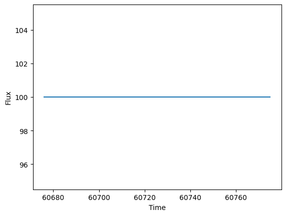
In the most basic form, the microlensing effect can be added to any model (BasePhysicalModel). Here we start with a constant SED model with no microlensing. As the name implies, the constant SED model will produce constant flux values for all times and wavelengths.

# Define the source model with a constant SED of 100.
source = ConstantSEDModel(brightness=100.0)

# Set some times and a single wavelength on which to evaluate the source SED.
t_start = 60676.0
times = np.arange(100.0) + t_start
wavelengths = np.array([7000.0])
fluxes = source.evaluate_sed(times, wavelengths)

# Plot the resulting lightcurve.
plt.plot(times, fluxes)
plt.xlabel("Time")
plt.ylabel("Flux")
plt.show()

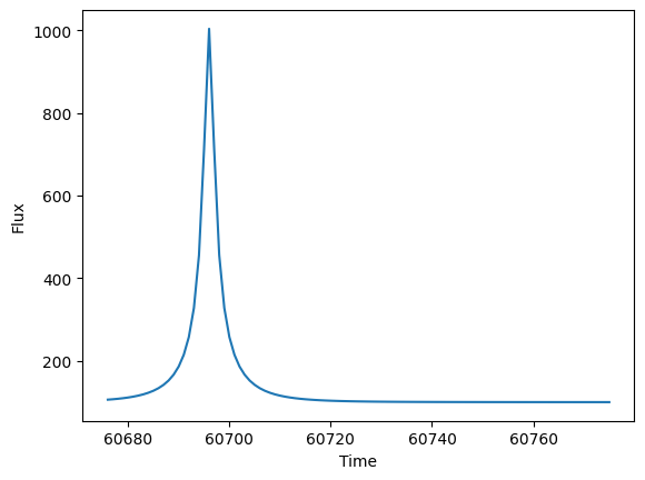
Now we add a microlensing effect. We do this by defining the microlensing effect and its parameters, then add the effect to the source model with add_effect(). Note, as we will show below, the parameters for the effect can be set the same way as the source’s parameters (constants, sampled from a distribution, computed from a function, etc.).

As you can see, the microlensing introduces a magnification 20.0 days after the start of the light curve.

ml_effect = Microlensing(microlensing_t0=t_start + 20.0, u_0=0.1, t_E=10.0)
source.add_effect(ml_effect)

fluxes = source.evaluate_sed(times, wavelengths)

plt.plot(times, fluxes)
plt.xlabel("Time")
plt.ylabel("Flux")
plt.show()

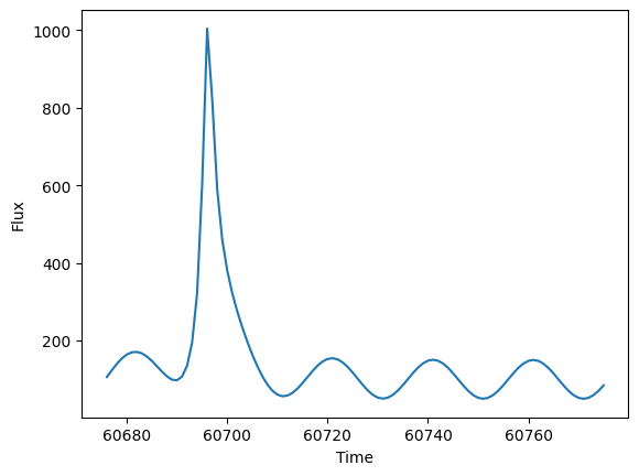
The model underneath the microlense does not need to be constant. We could simulate a small amount of variability by using a sin wave based model.

source2 = SinWaveModel(brightness=100.0, amplitude=50.0, frequency=0.05, t0=t_start)
source2.add_effect(ml_effect)
fluxes = source2.evaluate_sed(times, wavelengths)

plt.plot(times, fluxes)
plt.xlabel("Time")
plt.ylabel("Flux")
plt.show()

More Complex Models

We can extend the microlensing effect with any one of our SED or bandflux based models. For example consider a LightcurveModel which takes sample data points in each bandflux and returns the interpolated values.

We start by loading passbands, which are needed from the light curve model. Here we use (potentially older) data from the test directory to avoid needing to do a download. Users will generally want to download the most recent passbands. See the passbands notebook for more details.

# Load the passband data for the griz filters only.
filters = ["g", "r", "i", "z"]
passband_group = PassbandGroup.from_preset(
    preset="LSST",
    filters=filters,
    units="nm",
    trim_quantile=0.001,
    delta_wave=1,
    table_dir=data_dir / "passbands",
)

Next we define a series of light curves to use as our background model. These will be defined for the griz filters.

dts = np.arange(100.0)
times = dts + t_start

lightcurves = {
    "g": np.array([times, 3.0 * np.ones_like(times)]).T,  # Constant at 3.0
    "r": np.array([times, 0.02 * dts + 1.0]).T,  # Slight linear increase
    "i": np.array([times, np.sin(dts / 10.0) + 1.5]).T,  # Sin wave
    "z": np.array([times, 2.0 * np.ones_like(times)]).T,  # Constant at 2.0
}

lc_source = LightcurveTemplateModel(lightcurves, passband_group, t0=0, lc_data_t0=0)
graph_state = lc_source.sample_parameters(num_samples=1)

query_filters = np.array([filters[i % 4] for i in range(len(times))])
fluxes = lc_source.evaluate_bandfluxes(passband_group, times, query_filters, graph_state)

plot_lightcurves(fluxes, times, fluxerrs=None, filters=query_filters)

<Axes: xlabel='Time (MJD)', ylabel='Flux (nJy)'>

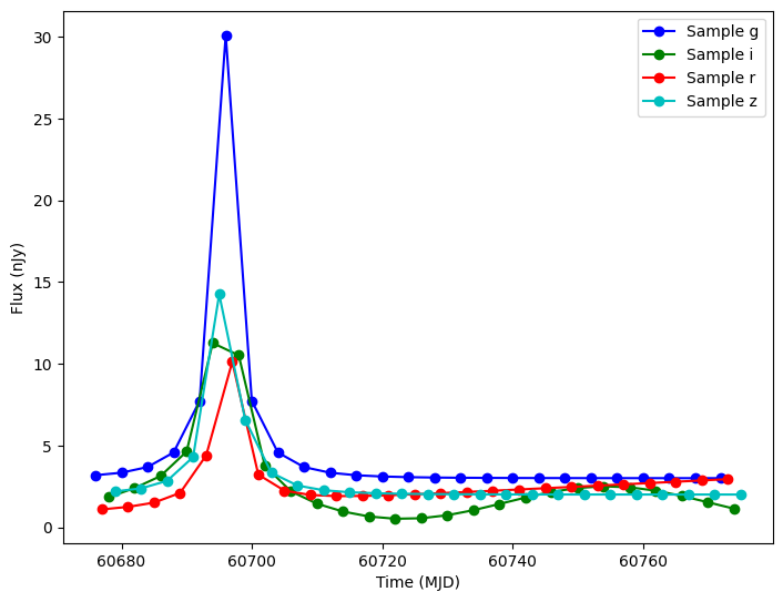
We can add microlensing to this model as we would any other model.

lc_source.add_effect(ml_effect)

# We need to resample to include the effect’s parameters.
graph_state = lc_source.sample_parameters(num_samples=1)
fluxes = lc_source.evaluate_bandfluxes(passband_group, times, query_filters, graph_state)

plot_lightcurves(fluxes, times, fluxerrs=None, filters=query_filters)

<Axes: xlabel='Time (MJD)', ylabel='Flux (nJy)'>

Varying the Microlensing Parameters

The main parameters of the microlensing model (microlensing_t0, u_0, and t_E) can be set like any other sample-able parameter. For example, let’s draw the start time uniformly from [60686.0, 60700.0], u_0 from a normal centered on 0.1, and t_E from a normal centered on 20.0. We can then draw 10 samples and see how they vary.

source = ConstantSEDModel(brightness=100.0, node_label="source")

ml_effect = Microlensing(
    microlensing_t0=NumpyRandomFunc("uniform", low=60686.0, high=60700.0),
    u_0=NumpyRandomFunc("normal", loc=0.1, scale=0.01),
    t_E=NumpyRandomFunc("normal", loc=20.0, scale=3.0),
)
source.add_effect(ml_effect)

state = source.sample_parameters(num_samples=5)

print("T0:", state["source"]["microlensing_t0"])
print("u_0:", state["source"]["u_0"])
print("t_E:", state["source"]["t_E"])

T0: [60686.98548745 60688.72945441 60686.0604508  60690.43909128
 60695.40213354]
u_0: [0.11570889 0.09995523 0.11149132 0.09009838 0.0973346 ]
t_E: [18.76494889 22.09156345 10.63592725 15.6548989  19.2568929 ]

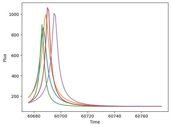
And we can plot the first few curves. Notice how the timing and shape of the lensing event varies.

fluxes = source.evaluate_sed(times, wavelengths, graph_state=state)

for i in range(5):
    plt.plot(times, fluxes[i, :, 0])
plt.xlabel("Time")
plt.ylabel("Flux")
plt.show()

Probabilistically Applying Microlensing

The microlensing effect also includes the ability to probabilistically apply the effect to only a subset of the light curves. This is useful if you want a random 1 in every 10,000 stars to be microlensed. The probability is controlled via the probability parameter.

In the below example, only 50% of the samples will have the microlensing applied. The samples with microlensing are shown in red and the samples without it are shown in blue.

source = ConstantSEDModel(brightness=100.0, node_label="source")

ml_effect = Microlensing(
    microlensing_t0=NumpyRandomFunc("uniform", low=60686.0, high=60700.0),
    u_0=NumpyRandomFunc("normal", loc=0.1, scale=0.01),
    t_E=NumpyRandomFunc("normal", loc=20.0, scale=3.0),
    probability=0.5,
)
source.add_effect(ml_effect)

state = source.sample_parameters(num_samples=10)
fluxes = source.evaluate_sed(times, wavelengths, graph_state=state)
for i in range(10):
    if state["source"]["apply_microlensing"][i]:
        plt.plot(times, fluxes[i, :, 0], color="red")
    else:
        plt.plot(times, fluxes[i, :, 0], color="blue")
plt.xlabel("Time")
plt.ylabel("Flux")
plt.show()

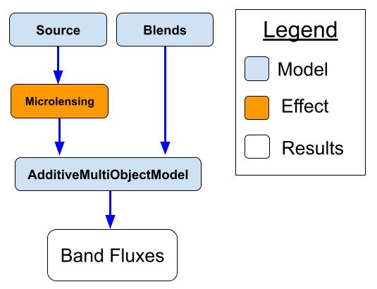
Blended Models

For a more realistic simulation, let us consider the combination of two different sources of flux:

• Source - The source that is being microlensed. This flux will be magnified by the lense.

• Blends - The flux coming from the background (or maybe the lense itself)

The structure of this model is shown in the following illustration:

from lightcurvelynx.models.multi_object_model import AdditiveMultiObjectModel

# Create the blends.
blends = ConstantSEDModel(brightness=50.0, node_label="blends")

# Create the model and add the lensing effect.
source = ConstantSEDModel(brightness=100.0, node_label="source")
ml_effect = Microlensing(microlensing_t0=t_start + 20.0, u_0=0.1, t_E=10.0)
source.add_effect(ml_effect)

# The full model is the sum of all three flux sources.
model = AdditiveMultiObjectModel([source, blends])

# Evaluate the combined model at different times.
fluxes_all = model.evaluate_sed(times, wavelengths)
fluxes_source = source.evaluate_sed(times, wavelengths)
fluxes_blends = blends.evaluate_sed(times, wavelengths)

plt.plot(times, fluxes_all, label="Combined Model")
plt.plot(times, fluxes_source, label="Source Model")
plt.plot(times, fluxes_blends, label="Blends Model")
plt.xlabel("Time")
plt.ylabel("Flux")
plt.legend()
plt.show()

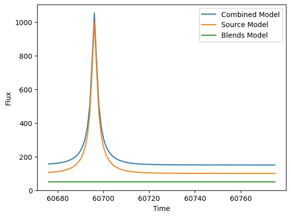
As we can see from the graph, in this example, the microlensing magnification was only applied to the source model (not the blends model).