EzTaoX Example

In this notebook we look at how we can import and use models from EzTaoX, a package for simulating and analyzing AGNs.

Note that the eztaox package is not installed as part of the default LightCurveLynx installation and currently has some version conflicts with other optional packages for LightCurveLynx. Users will need to manually install eztaox via pip (e.g. pip install eztaox) in order to run this notebook.

Dependency Conflicts:

If you run into dependency conflicts with JAX, you may be able to get around them by building extaox locally in the same virtual environment. To do this, clone the eztaox repository and make the following changes to its pyproject.toml:

• requires-python = ">=3.10, <3.13" -> requires-python = ">=3.10"

• "jax (==0.4.31)", -> "jax",

• "jaxlib (==0.4.31)", -> "jaxlib",

• "jaxopt (>=0.8.3,<0.9.0)", -> "jaxopt",

And recompile with pip install -e . in the extaox directory. Note that the JAX dependency constraints in extaox are due to some performance regressions. By downgrading the JAX library some of extaox’s functionality will run slower.

import numpy as np
import matplotlib.pyplot as plt

import eztaox.kernels.quasisep as ekq

from lightcurvelynx.math_nodes.basic_math_node import BasicMathNode
from lightcurvelynx.math_nodes.np_random import NumpyRandomFunc
from lightcurvelynx.obstable.opsim import OpSim
from lightcurvelynx.simulate import simulate_lightcurves
from lightcurvelynx.survey_info import SurveyInfo
from lightcurvelynx.models.eztaox_models import EzTaoXWrapperModel
from lightcurvelynx.utils.plotting import plot_lightcurves

Create the Survey Data

First we will load the survey information, which consists of the observations (obstable), passband information, and noise model. In this example, we create a fake OpSim that observes the exact same location on the sky (45.0, -20.0) three times a night, once in each of the ‘r”, “g”, and ‘i’ bands. This is not particularly realistic for a survey, but provides densely sampled output curves for the purpose of this notebook. For examples of more realistic RA/dec distributions and opsims, see the other notebooks.

Note that we specify a lot of noise parameters with the fake OpSim, but in normal cases users will be loading a predefined opsim with all of that information pre-populated.

Since we are using a standard survey type (LSST), we can just pass the name to the SurveyInfo info constructor and have it load the default passbands and noise model.

filters = ["g", "r", "i"]

num_days = 2000
mjd_start = 60676.0
mjd_end = mjd_start + num_days

num_samples = 50
survey_data = {
    "observationStartMJD": np.linspace(mjd_start, mjd_end, num_samples),
    "fieldRA": np.full(num_samples, 45.0),
    "fieldDec": np.full(num_samples, -20.0),
    "zp_nJy": np.random.normal(loc=1.0, scale=0.1, size=num_samples),
    "filter": [filters[i % 3] for i in range(num_samples)],
    "seeing": np.random.normal(loc=1.1, scale=0.1, size=num_samples),
    "skybrightness": np.random.normal(loc=20.0, scale=0.1, size=num_samples),
    "exptime": np.full(num_samples, 30.0),
    "nexposure": np.full(num_samples, 2),
}
obs_table = OpSim(survey_data)

survey_info = SurveyInfo(obstable=obs_table, survey_name="LSST")

Create the model

Next we want to create a model of the physical phenomena that we would like to simulation (in this case an AGN). EzTaoX uses a kernel to model an AGN event and provides a variety of built-in kernel types. We start with a simple exponential kernel (damped random walk model), which has two parameters scale and sigma. When creating a new kernel we need to provide dummy initial values (these won’t actually be used).

kernel = ekq.Exp(scale=1, sigma=1)

Next we need to define the parameters for the kernel and the Gaussian process simulation.

ExTaoX performs a simulation that accounts for the different in bands, so will we need to tell the code which bands we are using (and their order). We use the same three bands as defined above (filters list).

Kernel Parameters

The kernel parameters are the same as used in the object construction and are passed as a vector of log values with the order matching that of the constructor. Here we use a combination of LightCurveLynx’s built-in math nodes and numpy sampling nodes to create samplers. Each of these samplers will first sample a number from a uniform distribution and then apply the logarithm. So the values accessed during the simulation (and fed into MultiVarSim) will be log values.

log_kernel_param = [
    BasicMathNode("log(scale)", scale=NumpyRandomFunc("uniform", low=1.0, high=1000.0, node_label="scale")),
    BasicMathNode("log(sigma)", sigma=NumpyRandomFunc("uniform", low=0.01, high=1.0, node_label="sigma")),
]

This array now contains two LightCurveLynx samplers. The first will sample a scale uniformly from [1.0, 10000.0] and produce the log of that value. The second will sample a sigma uniformly from [0.01, 2.0] and produce the log of that value.

GP Parameters

In addition the Gaussian process can take arrays of setters for log_amp_scale (length N), mean (length N-1), and lag (length N) where N is the number of filters. Only log_amp_scale is required. The other two are optional.

Here we provide precomputed fixed values of the log_amp_scale corresponding to amp_scales of 1.0, 0.8, and 0.5. Alternative we could specify the log_amp_scale as a list of NumpyRandomFunc. We could set up mean and lag arrays with similar approaches.

log_amp_scale = [0.0, -0.22, -0.69]

When using zero_mean the EzTaoX’s Gaussian Process will simulate the change in magnitude. To be meaningful we need an initial (baseline) magnitude for the AGN. We specify this in a dictionary mapping filter name to the baseline magnitude.

Again these can be any setter accepted by LightCurveLynx. Maybe we want to use constants for each AGN. Or baselines sampled from a distribution. We can even mix and match the setter types per-band.

baseline_mags = {
    "g": NumpyRandomFunc("normal", loc=23.0, scale=0.5),  # Gaussian around 23 mag
    "r": NumpyRandomFunc("normal", loc=23.0, scale=0.5),  # Gaussian around 23 mag
    "i": 23.0,  # Fixed baseline mag for i-band
}

Other Object Parameters

In addition to the EzTaoX parameters, we need the standard parameters for a physical model such as RA, dec, and redshift.

• RA drawn uniformly from [44.0, 46.0]

• DEC drawn uniformly from [-19.0, -21.0]

• redshift drawn uniformly from [0.01, 0.5]

Since the field of view of a Rubin observation has a radius of 1.75 degrees, we can sample RA and DEC for our observations from a small region around the center of the image and know they will show up in all the images.

ra_sampler = NumpyRandomFunc("uniform", low=44.0, high=46.0)
dec_sampler = NumpyRandomFunc("uniform", low=-21.0, high=-19.0)
redshift_sampler = NumpyRandomFunc("uniform", low=0.01, high=0.5)

Model Creation

Now we are ready to create the model.

source = EzTaoXWrapperModel(
    kernel,  # The kernel to use
    baseline_mags=baseline_mags,  # A dict of baseline magnitude setters per band
    band_list=filters,  # A list of band names in order
    log_kernel_param=log_kernel_param,  # A list of setters for the kernel parameters
    log_amp_scale=log_amp_scale,  # A length N list of setters for the amplitude scales per band
    zero_mean=True,
    has_lag=False,
    ra=ra_sampler,
    dec=dec_sampler,
    redshift=redshift_sampler,
    node_label="source",  # A node name for convenience
)

Almost all of the parameters are randomly sampled. Let’s look at a sampling.

sampled_state = source.sample_parameters(num_samples=1)

for key, val in sampled_state["source"].items():
    print(f"{key}: {val}")

ra: 45.579647412319275
dec: -20.543939106173184
redshift: 0.1521399288891409
t0: None
distance: None
eztaox_log_kernel_param_0: 6.580064245876825
eztaox_log_kernel_param_1: -1.0076354490925996
eztaox_log_amp_scale_0: 0.0
eztaox_log_amp_scale_1: -0.22
eztaox_log_amp_scale_2: -0.69
eztaox_baseline_mag_g: 22.58944442772276
eztaox_baseline_mag_r: 23.285682457755804
eztaox_baseline_mag_i: 23.0
eztaox_seed_param: 3364319418

If we sample again, we get different values (except for the baseline in i band, which is fixed at 23.0)

sampled_state = source.sample_parameters(num_samples=1)

for key, val in sampled_state["source"].items():
    print(f"{key}: {val}")

ra: 45.51088875479686
dec: -19.51416993799136
redshift: 0.365701676074277
t0: None
distance: None
eztaox_log_kernel_param_0: 6.390081531313291
eztaox_log_kernel_param_1: -0.33546985995099543
eztaox_log_amp_scale_0: 0.0
eztaox_log_amp_scale_1: -0.22
eztaox_log_amp_scale_2: -0.69
eztaox_baseline_mag_g: 21.961499914436324
eztaox_baseline_mag_r: 23.27364511558056
eztaox_baseline_mag_i: 23.0
eztaox_seed_param: 1915706631

Generate the simulations

We can now generate random simulations with all the information defined above. The simulate_lightcurves function takes several parameters: the source from which we want to sample (here the collection of lightcurves), the number of results to simulate (100), and the survery information.

lightcurves = simulate_lightcurves(source, 5, survey_info)

Simulating: 100%|██████████| 5/5 [00:01<00:00,  3.76obj/s]

The results are written in the nested-pandas format for easy analysis. Each row corresponds to a single simulated object, with a unique id, ra, dec, etc. The column params include all internal state, including hyperparameter settings, that was used to generate this object. The nested lightcurve column contains the times, filters, and fluxes for each observation of that object. We can treat it as a (nested) table.

Let’s look at the lightcurve for the first object sampled:

print(lightcurves.loc[0]["lightcurve"])

             mjd filter         flux     fluxerr  flux_perfect  survey_idx  \
0   60676.000000      g  1902.572908  298.084163   1530.171474           0
1   60716.816327      r  3975.372974  322.427052   4072.982084           0
..           ...    ...          ...         ...           ...         ...
48  62635.183673      g  1587.161349  355.046633   1843.537672           0
49  62676.000000      r  5703.261291  361.184583   5419.256035           0

    obs_idx  is_saturated
0         0         False
1         1         False
..      ...           ...
48       48         False
49       49         False

[50 rows x 8 columns]

Let’s see where we generated the observations by using the results RA and dec columns. As expected the are within a box in the center of the field of view.

plt.plot(lightcurves["ra"], lightcurves["dec"], ".")
plt.xlabel("RA (deg)")
plt.ylabel("Dec (deg)")
plt.gca().invert_xaxis()
plt.title("Simulated Event Positions")
plt.show()

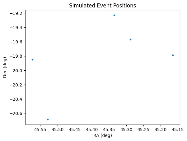
As noted above, these points are all clustered within the single viewing window of the survey so that we can get dense curves.

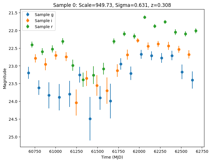
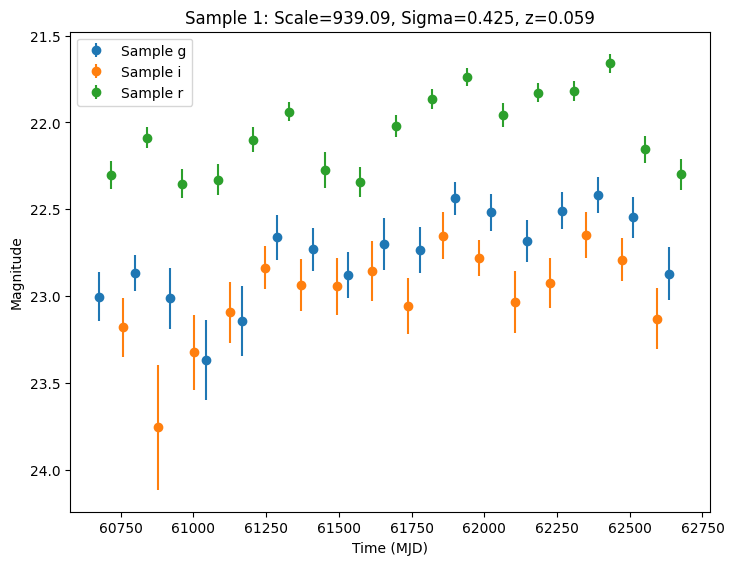
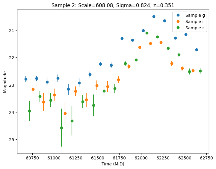
Now let’s plot the first few lightcurves to see what they look like when observed via Rubin’s cadence. We plot the results in magnitudes to be consistent with EZTaoX outputs. However note that our error bars can be huge for small fluxes (and this is something we need to fix).

for idx in range(3):
    # Extract the row for this object.
    lc = lightcurves.loc[idx]

    if lc["nobs"] == 0:
        continue

    # Unpack the nested columns (filters, mjd, flux, and flux error).
    lc_filters = np.asarray(lc["lightcurve"]["filter"], dtype=str)
    lc_mjd = np.asarray(lc["lightcurve"]["mjd"], dtype=float)
    lc_flux = np.asarray(lc["lightcurve"]["flux"], dtype=float)
    lc_fluxerr = np.asarray(lc["lightcurve"]["fluxerr"], dtype=float)

    scale = np.exp(lc["params"]["source.eztaox_log_kernel_param_0"])
    sigma = np.exp(lc["params"]["source.eztaox_log_kernel_param_1"])
    redshift = lc["params"]["source.redshift"]

    # Plot the lightcurves.
    ax = plot_lightcurves(
        fluxes=lc_flux,
        times=lc_mjd,
        fluxerrs=lc_fluxerr,
        filters=lc_filters,
        title=f"Sample {idx}: Scale={scale:.2f}, Sigma={sigma:.3f}, z={redshift:.3f}",
        plot_magnitudes=True,
    )
    ax.legend()
    plt.show()

Setting the Seed

As described in the LightCurveLynx documentation, it is possible to force deterministic behavior for debugging by passing a random number generator to the sampling or simulation functions. However, this only addresses the randomness during parameter sampling.

The EZTaoX code itself uses randomness when simulating the AGN. We can force deterministic behavior using the class’s seed_param argument when constructing the object (e.g. seed_param=42).

NOTE: This should only be done for testing. For actual scientific analysis, you will want actual random behavior.

Validating with EZTaoX

We can compare the simulated light curves with the results coming directly from the EZTaoX module. We need to set up an equivalent EZTaoX simulation, so we start by extracting the parameters that used from the saved parameters (from the “params” column in the results). We can then get the parameters using a combination of node name and the parameter name.

import jax.numpy as jnp

params = lightcurves.loc[0]["params"]

# The sampled values from a NumpyRandomFunc are stored in the "function_node_result" parameter by
# default, so we can extract the values used for sigma and scale.
sigma = params["sigma.function_node_result"]
scale = params["scale.function_node_result"]
print(f"Using scale={scale:.2f} and sigma={sigma:.3f} for the kernel parameters.")

# We can reuse the log_amp_scale directly since they are fixed in this example.
print(f"Using log_amp_scale={log_amp_scale} for the amplitude scaling.")

# Compile the initial parameters in a dictionary (making everything a JAX array).
init_params = {
    "log_kernel_param": jnp.array([np.log(scale), np.log(sigma)]),
    "log_amp_scale": jnp.array(log_amp_scale),
}

Using scale=949.73 and sigma=0.631 for the kernel parameters.
Using log_amp_scale=[0.0, -0.22, -0.69] for the amplitude scaling.

We copy the baseline magnitudes from their saved entries in the source node.

baselines = {}
for f in filters:
    baselines[f] = params[f"source.eztaox_baseline_mag_{f}"]
    print(f"Using baseline magnitude {baselines[f]:.2f} for filter {f}.")

Using baseline magnitude 23.40 for filter g.
Using baseline magnitude 22.44 for filter r.
Using baseline magnitude 23.00 for filter i.

Finally, we copy the random seed used for the AGN simulation, so we can run the same simulation.

jax_seed = params["source.eztaox_seed_param"]
print(f"Reusing seed={jax_seed}")

Reusing seed=3858143933

We extract the times for the simulation from the survey data. We also create a mapping from the filter name (in survey_data to the corresponding index).

import jax.numpy as jnp

times = jnp.array(survey_data["observationStartMJD"])
times_0 = times - jnp.min(times)  # Shift times to start at 0.

filter_list = np.array(survey_data["filter"])
filter_index_map = {"g": 0, "r": 1, "i": 2}
filter_indices = jnp.array([filter_index_map[filt] for filt in filter_list])

# Display the first 5 entries to verify the time and filter index mapping.
for i in range(5):
    print(
        f"Time: {times_0[i]:.2f} days, Filter: {survey_data['filter'][i]}, Filter Index: {filter_indices[i]}"
    )

Time: 0.00 days, Filter: g, Filter Index: 0
Time: 40.82 days, Filter: r, Filter Index: 1
Time: 81.63 days, Filter: i, Filter Index: 2
Time: 122.45 days, Filter: g, Filter Index: 0
Time: 163.27 days, Filter: r, Filter Index: 1

from eztaox.simulator import MultiVarSim
import jax

# Use the same kernel type as the source model.
kernel2 = ekq.Exp(scale=1, sigma=1)

# Create the simulator object using the given parameters and run it.
sim = MultiVarSim(
    kernel2,
    0.01,
    np.max(times_0),  # The last time to simulate.
    3,  # The number of bands to simulate.
    init_params=init_params,
    zero_mean=True,
    has_lag=False,
)

# Simulate ALL the times and bands at once by passing in the full arrays of times and band indices.
_, direct_mags = sim.fixed_input_fast(
    (times_0, filter_indices),  # Tuple of times and band indices
    jax.random.PRNGKey(jax_seed),  # Use the per-run seed.
)

Now we can compare the results for the direct simulation with the results from LightCurveLynx. There are a few places where we need to be careful: 1) the results from LightCurveLynx are in fluxes and need to be transformed to magnitudes. 2) The LightCurveLynx simulation also applied a baseline magnitude.

from lightcurvelynx.astro_utils.mag_flux import flux2mag

# We use the noisefree fluxes from the lightcurves and convert them to magnitudes
# for comparison with the direct simulation.
lcl_fluxes = np.asarray(lightcurves.loc[0]["lightcurve"]["flux_perfect"], dtype=float)
lcl_mags = flux2mag(lcl_fluxes)

# Convert direct magnitudes to numpy array for easier indexing.
direct_mags = np.array(direct_mags)

for filt in filters:
    # Select the values for the current filter.
    filter_mask = np.array(survey_data["filter"]) == filt
    lcl_vals = lcl_mags[filter_mask]

    # Add the baseline values to the direct simulation magnitudes for comparison.
    direct_vals = direct_mags[filter_mask] + baselines[filt]

    diffs = lcl_vals - direct_vals
    print(
        f"Filter {filt}: Mean difference = {np.mean(diffs):.4f} mag, Max difference = {np.max(diffs):.4f} mag"
    )

Filter g: Mean difference = 0.0000 mag, Max difference = 0.0000 mag
Filter r: Mean difference = 0.0000 mag, Max difference = 0.0000 mag
Filter i: Mean difference = 0.0000 mag, Max difference = 0.0000 mag