LightcurveTemplateModel Demo

The LightcurveTemplateModel model is designed to replicate given light curves in specific bands. It is specified as a separate light curve for each passband. In this notebook we provide an introductory demo to setting up and using the LightcurveTemplateModel model.

If you are interested in simulating curves of full SEDs over time, use the SEDTemplateModel or MultiSEDTemplateModel instead.

Setup

import matplotlib.pyplot as plt
import numpy as np

from lightcurvelynx.astro_utils.passbands import PassbandGroup
from lightcurvelynx.consts import lsst_filter_plot_colors
from lightcurvelynx.models.lightcurve_template_model import (
    LightcurveBandData,
    LightcurveTemplateModel,
    MultiLightcurveTemplateModel,
)

/home/docs/checkouts/readthedocs.org/user_builds/lightcurvelynx/envs/latest/lib/python3.12/site-packages/tqdm/auto.py:21: TqdmWarning: IProgress not found. Please update jupyter and ipywidgets. See https://ipywidgets.readthedocs.io/en/stable/user_install.html
  from .autonotebook import tqdm as notebook_tqdm

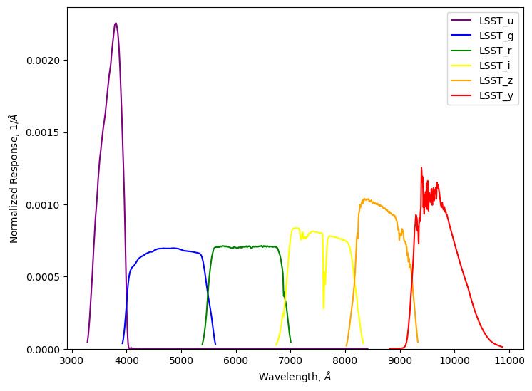
We start be loading the passbands that we will use to define the model. In this case we use the passbands from the LSST preset (but use a cached local version in the test directory to avoid a download). In most cases users will want to use data/passbands/ from the root directory.

# Use a (possibly older) cached version of the passbands to avoid downloading them.
table_dir = "../../tests/lightcurvelynx/data/passbands"
passband_group = PassbandGroup.from_preset(preset="LSST", table_dir=table_dir)
filters = passband_group.filters
print(passband_group)

wavelengths = passband_group.waves
min_wave, max_wave = passband_group.wave_bounds()
print(f"Wavelengths range [{min_wave}, {max_wave}]")

passband_group.plot()

PassbandGroup containing 6 passbands: LSST_u, LSST_g, LSST_r, LSST_i, LSST_z, LSST_y
Wavelengths range [3285.0000000000646, 10875.00000000179]

Creating the model

We create the model from light curves for each passbands of interest. This is what we want the model to reproduce then we call evaluate_bandfluxes(). While these light curves do no need to be the same as in the PassbandGroup every light curve must have a corresponding entry in the PassbandGroup.

The times of a light curve are defined relative to a reference epoch. In some cases the reference epoch will be the first time in the input data, indicating that the light curve starts at the first data point. In other cases users might want to set the reference epoch as the actual start of the event in the light curve or the peak of the event. It will depend on what is being simulated.

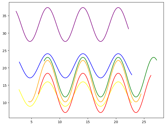
For simplicity of the demo, we create each curve as a randomly parameterized sin wave. Note that the times for all the light curves do not need to be the same.

num_times = 100
times = np.linspace(0, 20, num_times)

lightcurves = {}
for filter in filters:
    amp = 5.0 * np.random.random() + 1.0
    flux_offset = np.random.random() * 25 + 10
    time_offset = np.random.random() * 10
    filter_flux = amp * np.sin(times + time_offset) + flux_offset
    print(f"Filter {filter}: {amp:.2f} * sin(t + {time_offset:.2f}) + {flux_offset:.2f}")

    lightcurves[filter] = np.array([times + time_offset, filter_flux]).T

Filter u: 4.90 * sin(t + 2.25) + 32.47
Filter g: 3.50 * sin(t + 2.82) + 20.57
Filter r: 5.73 * sin(t + 7.24) + 17.31
Filter i: 3.54 * sin(t + 2.78) + 12.43
Filter z: 5.99 * sin(t + 4.47) + 16.15
Filter y: 5.68 * sin(t + 6.23) + 12.77

# Plot the light curves
figure = plt.figure()
ax = figure.add_axes([0, 0, 1, 1])
for filter, lightcurve in lightcurves.items():
    color = lsst_filter_plot_colors.get(filter, "black")
    ax.plot(lightcurve[:, 0], lightcurve[:, 1], color=color, label=filter)

We then create the model from the dictionary of light curve information.

In addition to the light curve data itself, the model also needs to know:

• t0 - The survey date (e.g. in MJD) that corresponds to the model’s reference epoch.

• lc_data_t0 - The time stamp of the input data (lightcurves) specifying the model’s reference epoch. If the survey made an observation at time t0, it would measure the band flux corresponding to the lc_data_t0 timestamp.

The difference between lc_data_t0 and t0 is needed due to how the data can be provided. For example we could read in simulated supernova curve that starts at MJD 59534.5, but latter simulate the same light curve starting at t0=63426.0. In this case we would need to set lc_data_t0=59534.5 to indicate that our supernova light curve starts then (alternative we could use a later time if we want the reference epoch to correspond to the peak of the light curve). We would set t0=63426.0 to indicate that this is where we want to add the light curve to the new simulation.

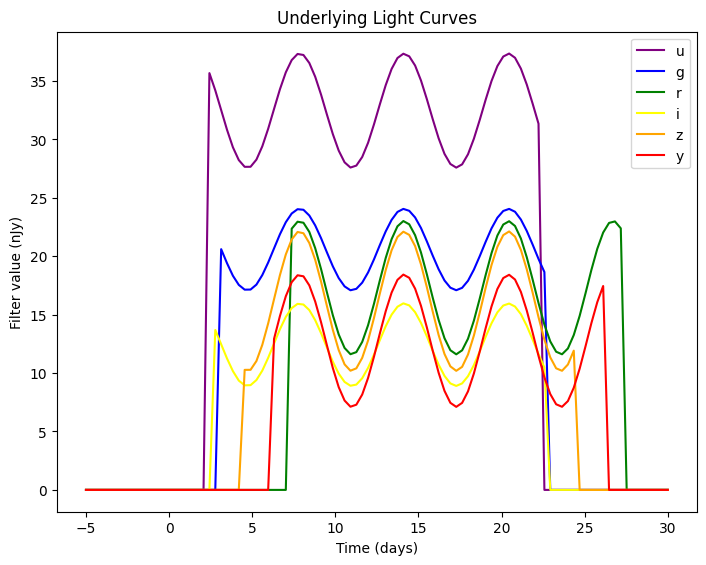
model = LightcurveTemplateModel(lightcurves, passband_group, lc_data_t0=0.0, t0=0.0)

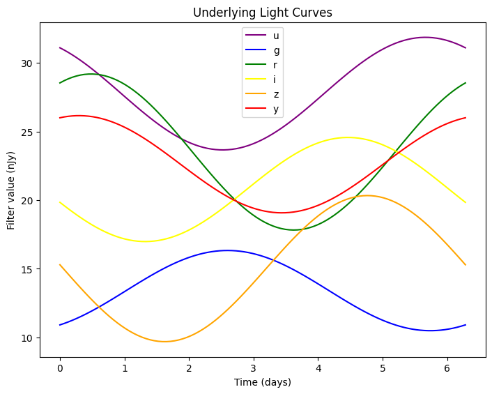
If we plot the underlying light curves we can see they matched the provided ones. Note that by definition non-periodic light curves drop to 0.0 outside their range. Later we will see how to set a baseline value.

plot_times = np.linspace(-5, 30, 100)
model.plot_lightcurves(times=plot_times)

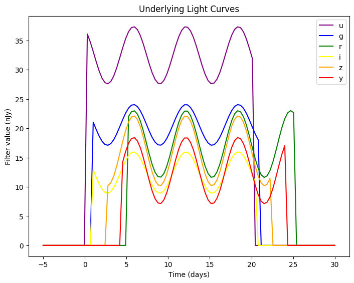
As described above, the reference epoch of a light curve indicates the time stamp from the incoming data that should correspond to the model’s t0. For example, if we set the reference epoch of the model to 2.0 the light curve will be shifted to the left so that a query time of 0.0 corresponds to the input data’s time stamp of 2.0.

model_shifted = LightcurveTemplateModel(lightcurves, passband_group, lc_data_t0=2.0, t0=0.0)
model_shifted.plot_lightcurves(times=plot_times)

Generating Bandfluxes

We evaluate the LightcurveTemplateModel model the same way we evaltuate any source model with functions such as evaluate_sed(), sample_parameters(), and evaluate_bandfluxes(). This model was specifically designed for the evaluate_bandfluxes() function, so we explore that below.

Specifically, because the models are defined at the filter level, we do not need to generate the underlying SEDs and integrate with the filters’ passbands. Instead the LightcurveTemplateModel object will compute the band fluxes directly from the underlying curves.

The evaluate_bandfluxes() function requires two arrays to determine how the source was observed: an array of times at which the observations occurred and a corresponding array of filters in which the observation was made.

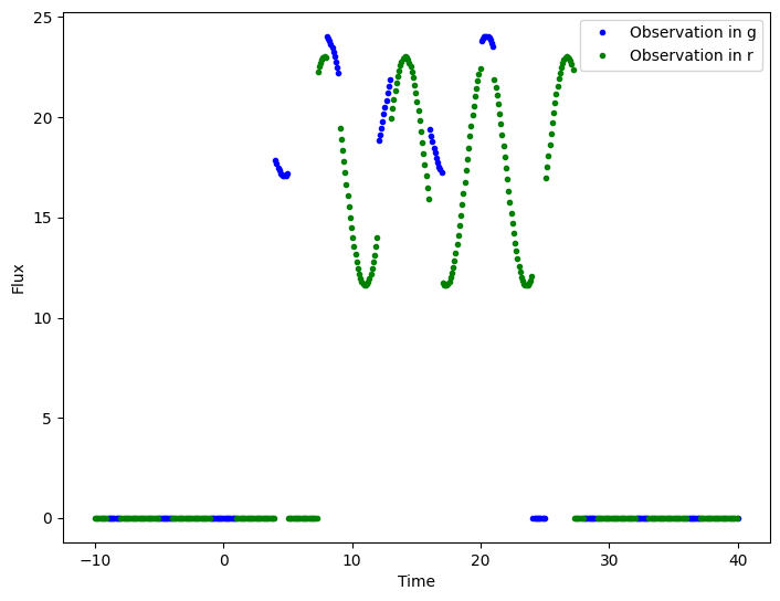
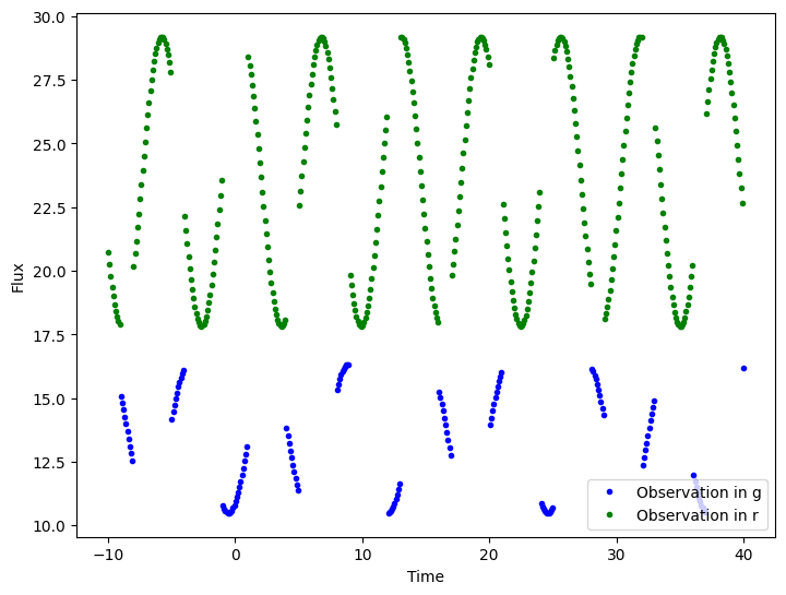
Let’s model a sequence of observations in the g and r filters only.

# The state is not used since we do not have any random parameters, but we need it for evaluate_bandfluxes().
state = model.sample_parameters(num_samples=1)

# Create query times over the middle of the range. Make 3/4 of them r and the rest g.
query_times = np.linspace(-10, 40, 500)
query_filters = np.array(["g" if int(t) % 4 == 0 else "r" for t in query_times])

# Get the fluxes for the query times and filters
flux = model.evaluate_bandfluxes(passband_group, query_times, query_filters, state)

/home/docs/checkouts/readthedocs.org/user_builds/lightcurvelynx/envs/latest/lib/python3.12/site-packages/lightcurvelynx/models/physical_model.py:969: UserWarning: Some times are less than the model's defined bounds and no time extrapolation is set. If this is not the intended, you can enable time extrapolation using the 'time_extrapolation' parameter.
  warnings.warn(
/home/docs/checkouts/readthedocs.org/user_builds/lightcurvelynx/envs/latest/lib/python3.12/site-packages/lightcurvelynx/models/physical_model.py:993: UserWarning: Some times are greater than the model's defined bounds and no time extrapolation is set. If this is not the intended, you can enable time extrapolation using the 'time_extrapolation' parameter.
  warnings.warn(

def print_fluxes(query_times, query_filters, flux):
    """Display the fluxes for the given query times and filters.

    Parameters
    ----------
    query_times : np.ndarray
        The times at which the fluxes are queried.
    query_filters : np.ndarray
        The filters corresponding to the query times.
    flux : np.ndarray
        The flux values for the query times and filters.
    """
    # Plot the fluxes
    figure = plt.figure()
    ax = figure.add_axes([0, 0, 1, 1])
    for filter in ["g", "r"]:
        mask = query_filters == filter
        color = lsst_filter_plot_colors.get(filter, "black")
        label = f"Observation in {filter}"
        ax.plot(query_times[mask], flux[mask], color=color, label=label, linewidth=0, marker=".")

    ax.set_xlabel("Time")
    ax.set_ylabel("Flux")
    ax.legend()
    plt.show()


print_fluxes(query_times, query_filters, flux)

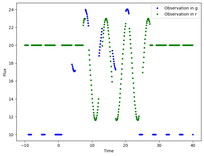
Setting Background Fluxes

For some light curves we might not want the default value to be 0.0. For example a variable star might have the value of 100.0 when active and 50.0 when inactive. We can set a baseline value for light curves using the baseline parameter. This parameter takes a dictionary mapping the filter name to the baseline value.

baseline = {
    "u": 0.0,
    "g": 10.0,
    "r": 20.0,
    "i": 30.0,
    "z": 40.0,
    "y": 50.0,
}

model = LightcurveTemplateModel(lightcurves, passband_group, lc_data_t0=0.0, t0=0.0, baseline=baseline)

# Evaluate the new model and plot the fluxes
state = model.sample_parameters(num_samples=1)
flux = model.evaluate_bandfluxes(passband_group, query_times, query_filters, state)
print_fluxes(query_times, query_filters, flux)

Periodic Models

LightcurveTemplateModel supports both periodic and non-periodic lightcurves. Periodic models require that each filter’s lightcurve is sampled at the same time and that the value at the end of the lightcurve is equal to the value at the start of the lightcurve. The lightcurve epoch (lc_t0) is automatically set to the first time so that the t0 parameter corresponds to the shift in phase.

num_times = 100
times = np.linspace(0, 2.0 * np.pi, num_times)

lightcurves = {}
for filter in filters:
    amp = 5.0 * np.random.random() + 1.0
    flux_offset = np.random.random() * 25 + 10
    phase_offset = np.random.random() * 10
    filter_flux = amp * np.sin(times + phase_offset) + flux_offset
    print(f"Filter {filter}: {amp:.2f} * sin(t + {phase_offset:.2f}) + {flux_offset:.2f}")

    lightcurves[filter] = np.array([times, filter_flux]).T

model = LightcurveTemplateModel(lightcurves, passband_group, lc_data_t0=0.0, t0=0.0, periodic=True)
model.plot_lightcurves()

Filter u: 4.10 * sin(t + 8.47) + 27.77
Filter g: 2.92 * sin(t + 5.26) + 13.41
Filter r: 5.69 * sin(t + 1.09) + 23.51
Filter i: 3.80 * sin(t + 3.39) + 20.78
Filter z: 5.33 * sin(t + 9.37) + 15.01
Filter y: 3.54 * sin(t + 7.56) + 22.62

# Evaluate the new model and plot the fluxes
state = model.sample_parameters(num_samples=1)
flux = model.evaluate_bandfluxes(passband_group, query_times, query_filters, state)
print_fluxes(query_times, query_filters, flux)

Multi-Lightcurve Models

Users can also load in a series of light curves and randomly (or programmatically) sample which light curve to use for each evaluation. The MultiLightcurveTemplateModel class takes in a list of LightcurveBandData with information about each light curve’s time range, values, periodicity, etc. Below we show an example of random sampling. See the “Simulating Known Objects” section for an example of programmatic sampling.

Unlike the LightcurveTemplateModel class, the MultiLightcurveTemplateModel class requires the user to provide the input as prepackaged LightcurveBandData objects. Here we create a source that randomly samples from two light curves. The first is a non-periodic light curve in u and g. The second is a periodic light curve in r and g. We provide weights so second light curve is more likely to be sampled than the first.

# Lightcurve 1 is non-periodic and covers u and g.
lc1_times = np.arange(0.0, 10.5, 0.5)
lc1_lightcurves = {
    "u": np.array([lc1_times + 0.1, 2.0 * np.ones_like(lc1_times)]).T,
    "g": np.array([lc1_times, 3.0 * np.ones_like(lc1_times)]).T,
}
lc1_data = LightcurveBandData(lc1_lightcurves, lc_data_t0=0.0, baseline={"u": 0.1, "g": 0.2})

# Lightcurve 2 is periodic and covers r and g.
lc2_times = np.arange(0.0, 19.0, 1.0)
lc2_lightcurves = {
    "r": np.array([lc2_times, lc2_times % 2]).T,
    "g": np.array([lc2_times, lc2_times % 2 + 0.5]).T,
}
lc2_data = LightcurveBandData(lc2_lightcurves, lc_data_t0=0.0, periodic=True)

# Create the MultiLightcurveTemplateModel with both light curves.
source = MultiLightcurveTemplateModel(
    [lc1_data, lc2_data],
    passband_group,
    weights=[0.3, 0.7],
    t0=0.0,
    node_label="source",
)

The light curve choosen for each evaluation is stored in the selected_lightcurve parameter.

state = source.sample_parameters(num_samples=10)
print(f"selected_lightcurve: {state['source']['selected_lightcurve']}")

selected_lightcurve: [1 1 1 1 1 1 0 1 1 0]

Simulating Known Objects

As mentioned in the previous section, the MultiLightcurveTemplateModel model can be used to programmatically evaluate a series of light curves. We do this by providing the indices (in order) of the light curves that we want to evaluate.

We can combine this approach with a TableSampler to sample a list of known light curves with other known parameters, such as position.

import pandas as pd
from lightcurvelynx.math_nodes.given_sampler import TableSampler

# Add a third light curve with r, g, u for the example.
lc3_times = np.arange(0.0, 11.5, 0.5)
lc3_lightcurves = {
    "u": np.array([lc3_times + 0.1, 2.0 * np.ones_like(lc3_times)]).T,
    "g": np.array([lc3_times, 3.0 * np.ones_like(lc3_times)]).T,
    "r": np.array([lc3_times, 1.0 * np.ones_like(lc3_times)]).T,
}
lc3_data = LightcurveBandData(lc3_lightcurves, lc_data_t0=0.0, baseline={"u": 0.1, "g": 0.2, "r": 0.3})

# Create a TableSampler with the light curve index, ra, and dec. We use in_order=True to
# sample each row exactly once and in order.
table = pd.DataFrame(
    {
        "lightcurve_index": [0, 1, 2],
        "ra": [10.0, 20.0, 30.0],
        "dec": [-10.0, -20.0, -30.0],
    }
)
sampler = TableSampler(table, in_order=True)

# Create the MultiLightcurveTemplateModel with parameters pulled from the TableSampler.
# For each sample the model with use the ra, dec, and light curve index from the same line.
source = MultiLightcurveTemplateModel(
    [lc1_data, lc2_data, lc3_data],
    passband_group,
    ra=sampler.ra,
    dec=sampler.dec,
    indices=sampler.lightcurve_index,
    t0=0.0,
    node_label="source",
)

# Note that we can sample *at most* 3 samples since there are only 3 lines in the table.
state = source.sample_parameters(num_samples=3)
for idx in range(3):
    print(
        f"Sample {idx}: lightcurve_index={state['source']['selected_lightcurve'][idx]}, "
        f"ra={state['source']['ra'][idx]}, dec={state['source']['dec'][idx]}",
    )

Sample 0: lightcurve_index=0, ra=10.0, dec=-10.0
Sample 1: lightcurve_index=1, ra=20.0, dec=-20.0
Sample 2: lightcurve_index=2, ra=30.0, dec=-30.0